Basic FDS Example I

Basic FDS Example I#

Simulation Setup Description#

As a basic example we create a FDS simulation setup with a simple propane gas burner. A soot yield of \(\mf 0.022~g/g\) is to be used. The gas burner shall have an edge length of \(\mf 0.4~m\) and should be raised \(\mf 0.2~m\) above the ground. It shall provide \(\mf 63~kW\) in a steady-state. The computational domain shall be \(\mf 2.0~m\) tall and have an extent of \(\mf 2.0~m\) in the x and y axis respectively. The fluid cells shall be cube-shaped with an edge length of \(\mf 0.2~m\). The overall simulation time should be \(\mf 60~s\).

For details on the pool fires and gas burners look at section Pool Fires.

FDS Input Files#

First you should create a new folder. In this directory the input file is to be saved later. All the generated output files will also be located here. It is useful to create individual directories for each simulation to not accidentially overwrite or mix up files. Create an empty plain text file. You could use any text editor (not a word processor) to create your text file. Although the file extenison does not matter, a common practice is to use the .fds extension.

The syntax of FDS input files is given by FORTRAN namelists. These namelists start with an ampersand & character and are followed by four capital letters. They end with a slash / character. Between these two, parameters of the respective namelist can be provided, for example:

&NAME P1=value P2=value /

The first entry in an FDS input file is &HEAD / and it ends with &TAIL /. In between head and tail of the file the definition of the simulation setup is provided by the user.

Note: The individual file paths are likely different on your system, depending on your file structure.

Meta Data of Simulation Setup (HEAD, TAIL)#

Now we will start defining the simulation setup. Two parameters that can be provided to the HEAD namelist are a character ID (CHID) and a title (TITLE). Both values are strings. The character ID is used to label all the files that are created during the simulation. It can be different from the file name of the FDS input file. As a short-hand, files are also referred to by using the CHID, for example CHID_devc.csv, since only the CHID-part is variable.

The title is a human-readable short description of the setup.

The file is closed out with TAIL.

Following the above, your input file should now contain the following lines:

&HEAD CHID  = 'Job_1', 
      TITLE = 'Our first FDS simulation' /

&TAIL /

Tip

CHID: is the character ID. This is the string used to tag the output files.
TITLE: is a descriptive text of your simulation.

Bounds of Time and Space (MESH, TIME)#

Time (TIME)#

The simulation time is specified in seconds, using the TIME namelist. The parameter T_END determines when the simulation ought to stop. Obviously, this is the time inside the simulation and not the time the computer takes to conduct the simulation, which would be referred to as “wall clock time”. The start time (T_BEGIN) could be adjusted as well, but this is seldom necessary, it is \(\mf 0~s\) by default. The input line should now look like this:

&TIME T_END = 60. /

Setting T_END = 0 will lead to FDS only setting up the simulation without running it. It also creates a Smokeview file, which can be used to check if everything is set up correctly.

Aditionally, the rate at which data is saved can be controlled, from the DUMP namelist. The parameter NFRAMES is used to divide the simulation time, i.e. T_END - T_BEGIN, into n frames. This is a global control, but different recording functions (DEVC, SLCF, etc.) can be controlled individually. Please refer to the users guide for detailed information how this can be achieved. To safe a single frame per second we use:

&DUMP NFRAMES=60 /

Tip

The grid and geometry can be checked in the following way:

Set T_END = 0, this will only build the geometry without actually running a simulation
Save the FDS input file
Run the FDS input file
Open the smokeview file (CHID.smv) and check the geometry
To display the grid, press g

Space (MESH)#

To conduct a simulation we need to define a computational domain and a time frame.

The domain is a rectangular cuboid shape that is divided in smaller volumes (cells) which are also rectangular cuboids, using the MESH namelist. It can be given a label (ID) to organise larger files with many MESHes. The domain volume is defined by providing coordinates of two points of opposing corners, see Fig. 2. They define the bounding box (XB) of the volume. Their values are to be provided in meters.

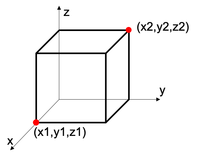
../../../_images/coordinates.png — Fig. 2 Coordinate definition for bounding boxes (`XB`) in FDS.#

The coordinates of the points are provided as a list of six values. At first the two x-coordinates, followed by the two y- and then the two z-coordinates, like this: XB = x1,x2, y1,y2, z1,z2,. In our example case the domain is supposed to be a cube with an edge length of \(\mf 2.0~m\). Let’s position it around the origin point in the x- and y-directions and start the z-axis at 0. This will lead to: XB = -1.00,1.00, -1.00,1.00, 0.00,2.00,.

The size of the fluid cells is indirectly defined, by dividing the domain along each axis. Thus, we need to provide integer values for each axis as the divisor. The parameter is IJK, where the “I” denotes the dividion along the x-axis, respectively “J” and “K” denote the y- and z-axis. Thus, getting to fluid cells of an edge length of \(\mf 0.2~m\), each domain edge needs to be divided by 10.

Combining all the above, the MESH definition should look like this:

&MESH ID  = 'Domain',
      IJK = 10,10,10,
      XB  = -1.00,1.00,-1.00,1.00,0.00,2.00 /

Obstruct the Flow Field (OBST)#

The flow field can be obstructed by using the OBST namelist. This essentially defines which cells are blocked for the flow field. For boundary conditions see section below.

FDS fundamentally works with a rectangular grid and all elements need to be aligned to it. This means essentially that all obstructions are rectangular objects as well. Right now, some effort is put into the development to allow non-rectangular objects (GEOM). Since this namelist is in active development, it will not be covered here.

To define the volume of an obstruction we use the same syntax for bounding boxes (XB), as described with the MESH above.

The initial description of the example simulation setup states that the burner shall have an edge length of \(\mf 0.4~m\) and be raised \(\mf 0.2~m\) off the ground. We accomplish this by using an obstruction, centered around the world origin. This should lead to the following line:

&OBST ID  = 'BurnerBase',
      XB  = -0.20,0.20,-0.20,0.20,0.00,0.20 /

Gas Phase Combustion (REAC)#

To initialise a fire, combustible gas needs to be introduced into the fluid domain. Its reaction is controlled using the REAC namelist.

FDS requires to be provided the stoichiometry of the gas phase combustion reactions. However, in a limited selection of cases the stoichiometry can be computed internally. This is also referred to as “simple chemistry”, see users guide for more details. FDS comes with a couple of predefined gaseous species, that can be found in “table 14.4: Pre-defined gas and liquid species” in the users guide. Combustible species listed there can be used with the simple chemistry, via the FUEL parameter.

Furthermore, a “surrogate fuel” concept is employed in FDS, together with the simple chemistry. It uses a single species for all gas phase combustion reactions, but scales their mass loss based on their respective heat of combustion. See “Chapter 15 Combustion” in the users guide.

Using the simple chemistry approach, yields of soot (SOOT_YIELD) and carbon monoxide (CO_YIELD) can be set. By default the yields are set to zero. Adding a soot yield will also lead to some indication of smoke in Smokeview.

Given the simulation setup description, the input line should look like this:

&REAC FUEL       = 'PROPANE',
      SOOT_YIELD = 0.022 /

Design Boundary Conditions (SURF)#

Obstructions define cells that are blocked for the flow field. Their surface also has an impact on the gas phase, for example due to heat transfer. This is controlled by defining and assigning boundary conditions. By default FDS assigns the INERT boundary condition, visualised by the yellow color.

Boundary conditions are called “surfaces” in FDS and are defined using the SURF namelist. Each surface definition needs to get a label (ID), which is used to connect it to the desired cells, i.e. obstructions or vents.

The SURF namelist, has a couple of special features to make life a bit easier for the user. There is a boolean flag to set a given surface as the default, conveniently called DEFAULT.

Tip

In FDS booleans can be used as a long or short form. The long form is encapsulated by periods “.”:

True: .TRUE. or T
False: .FALSE. or F

As some basic functionality, it can be used to change the color of boundaries. There are two options:

with COLOR one can access a bunch of labelled colors
with RGB three integers between 0 and 255 can be provided The predefined colors can be looked up in “Table 10.1: A sample of color definitions.” in the users guide.

Tip

Use colors at least during the design process of your simulation setup as a visual aid to make sure that individual boundary conditions are assigned to the correct places.

A Simple Gas Burner#

Furthermore, there is the HRRPUA parameter. It assignes a Heat Release Rate Per Unit Area as boundary conditions, in \(\mf kW/m^2\). It takes the surface area of the cells and scales the released combustible mass accordingly, see the pool fire section for more details. Now, to get our desired \(\mf 63~kW\) we need to divide it by the surface area of the burner. According to the description, the burner is a square with an edge length of \(\mf 0.4~m\). Thus, we compute the HRRPUA value \(\mf 63~kW / (0.4~m \times 0.4~m)\) to be about \(\mf 393.75~kW/m^2\).

Tip

In FDS OBST and VENT need to align to the MESH and it will adjust them to make it fit. Thus, check if the HRRPUA yields the expected HRR! (e.g. check CHID_hrr.csv file)

Let’s combine the above information to create the boundary condition of our gas burner:

&SURF ID     = 'Burner',
      COLOR  = 'RASPBERRY',
      HRRPUA = 393.74999999999994 /

Assign Boundary Conditions (VENT)#

There are different ways in FDS to assign boundary conditions to obstructions. Some short-hand solutions are available in the OBST definitions: SURF_ID, SURF_IDS and SURF_ID6. With SURF_ID all six sides of the rectangular cuboid are assigned the same boundary condition. A bit more granular is SURF_IDS, which allows access to the top, sides and bottom of an obstruction. Most granular is SURF_ID6, where all faces are accessible individually (-x, +x, -y, +y,-z, +z). For the last two options, arrays of strings are to be provided for each of the options, i.e. SURF_IDS = 'top', 'sides', 'bottom'.

In most cases an obstruction is covering many cells but only a subset of them should be assigned a specific boundary condition. This subset can be defined using the VENT namelist. In this example we use this to assign the burner boundary to the top of the obstruction defined above. To define the dimensions of the vent, we use the bounding box again, just set the hight to zero, i.e. z1 and z2 get the same value:

&VENT ID      = 'BurnerOutlet',
      SURF_ID = 'Burner',
      XB      = -0.20,0.20,-0.20,0.20,0.20,0.20 /

For now, the computational domain we set up is closed off, notice the yellow walls. Therefore, the combustion products will accumulate and eventually the fire will extinguish. Among the predefined boundary conditions is one called OPEN. We can use it on the domain (MESH) boundaries to allow gas to enter and leave the domain. FDS provides a convenience feature to select a face of the domain. For example the face in the positive x direction can be adressed by using XMAX, together with MB (mesh boundary) or DB (domain boundary). Be aware, this will adress the whole face. To open all sides and the top, use the following lines:

&VENT MB='XMIN', SURF_ID='OPEN' /
&VENT MB='XMAX', SURF_ID='OPEN' /
&VENT MB='YMIN', SURF_ID='OPEN' /
&VENT MB='YMAX', SURF_ID='OPEN' /

&VENT MB='ZMAX', SURF_ID='OPEN' /

Record Data (DEVC, SLCF)#

FDS has vast capabilities to record different data sets. Most of the data you would like to keep, you need to specifiy before the simulation is conducted. Here we provide only a very brief introduction to record data, for more details look into the other examples and the users guide. The focus is on devices DEVC and slices SLCF.

Devices (DEVC)#

To record the computed gas temperature above the burner we can use a point device (DEVC). A device can get a label (ID), which makes it much easier to identify in the comma separated value (CSV) file created during the simulation. It needs a location and a quantity.

Locations can be provided in different ways, we focus her on a single point using XYZ. However, lines, planes and volumes are possible as well.

The QUANTITY parameter expects a string to define what values are to be recorded. As an example, let’s take the gas temperature, using TEMPERATURE.

The input line could be looking like this:

&DEVC ID       = 'Temp_1m',
      XYZ      = 0.1, 0.1, 1.3,
      QUANTITY = 'TEMPERATURE' /

Tip

The quantity ‘TEMPERATURE’ is not a thermocouple! Also, it cannot be used for temperatures of a solid. Please, check the users guide.

Slices (SLCF)#

Many gas phase quantities can also be recorded as animated slices across the domain, using the SLCF namelist. The locations of the slices can be defined as planes, using for example the PBX parameter. This will create a plane which extents along the y- and z-axis, it will be moved along the x-axis (unit: meter). A quantity needs to be provided, here the gas temperature. Furthermore, the CELL_CENTERED flag can be set to force FDS to record data at the cell centeres. It will then also show up in Smokeview not as interpolated data. Below is an exaple input:

&SLCF PBX           = 0.00,
      QUANTITY      = 'TEMPERATURE',
      CELL_CENTERED = .TRUE. /

Tip

To get access to the ‘SLCF’ data, check out the Tools section about the fdsreader Python module.

File#

&HEAD CHID  = 'Ex1',
      TITLE = 'Basic Example 1 - Gas Burner' /

&TIME T_END = 60.0 /
&DUMP NFRAMES = 60 /

&MESH ID  = 'Domain',
      IJK = 10,10,10,
      XB  = -1.00,1.00,-1.00,1.00,0.00,2.00 /



# ---------------------------------------
# Domain boundary
# ---------------------------------------

&VENT MB='XMIN', SURF_ID='OPEN' /
&VENT MB='XMAX', SURF_ID='OPEN' /
&VENT MB='YMIN', SURF_ID='OPEN' /
&VENT MB='YMAX', SURF_ID='OPEN' /

&VENT MB='ZMAX', SURF_ID='OPEN' /



# ---------------------------------------
# Gas burner: propane
# ---------------------------------------

&SPEC ID = 'PROPANE' /

&REAC FUEL       = 'PROPANE',
      SOOT_YIELD = 0.022 /

# HRR: 62.9 kW
&SURF ID         = 'Burner',
      COLOR      = 'RASPBERRY',
      HRRPUA     = 393.74999999999994 /

&OBST ID      = 'BurnerBase',
      SURF_ID = 'INERT',
      XB      = -0.2, 0.2, -0.2, 0.2, 0.0, 0.2 /

&VENT ID      = 'BurnerOutlet',
      SURF_ID = 'Burner',
      XB      = -0.2, 0.2, -0.2, 0.2, 0.2, 0.2 /



# ---------------------------------------
# Analysis
# ---------------------------------------

&DEVC ID       = 'Temp_1m',
      XYZ      = 0.1, 0.1, 1.3,
      QUANTITY = 'TEMPERATURE' /


&SLCF PBX           = 0.00,
      QUANTITY      = 'TEMPERATURE',
      CELL_CENTERED = .TRUE. /



&TAIL /

Questions and Tasks#

How do you adjust the domain, that the fluid cells are cubes with an edge length of \(\mf 0.1~m\)?
Given the original MESH of the example above, what happens when you set the z2 coordinate of the ‘BurnerBase’ OBST to \(\mf 0.24~m\)?
Change the combustible gas to toluene.
Add a CO yield of 0.01 g/g.
Start from closed domain boundaries and open only a section on the face in the positive x direction, between the heights of \(\mf 0.6~m\) to \(\mf 1.6~m\).
Look up the COLOR = 'RASPBERRY' in the users guide and change it to its RGB value.
In your own words, explain the surrogate fuel concept in FDS.
Add a slice for gas temperatures on the y-axis at \(\mf 0.2~m\).
Add a slice that shows you the gas velocity.
Add a slice that allows you to determine that the CO yield works.
Add a slice that allows you to determine if toluene is introduced.