Example – Pool Fire

3.2. Example – Pool Fire#

Introduction#

Pool fires are interesting for studying fire development, because they are relatively easy to handle. One needs a fireproof pan, for example made out of steel sheets, and fill in a combustible liquid. Shortly after ignition, it reaches a quasi steady-state, due to the evaporation of the liquid. One of the shortcomings of pool fires is their limited fuel supply. This is one of the reasons why gas burners are often used in fire experiments. That, and the good reproducibility associated with gas burners as ignition source. Also in FDS, most pool fire simulations are modelled as gas burners (see Section “11.4 Simple Pyrolysis Models” in the FDS User’s Guide).

This example illustrates the setup and analysis of a minimalist FDS simulation. Starting from a simple pool fire with a fixed heat release rate, the model is extended by various parameters. The results are then validated by comparison with simple analytical methods.

Setup#

A pool fire scenario is considered as an example of a FDS simulation. The pool surface area is $\mf 1~m^2$ and it is located at $\mf z = 0$. The heat release rate of the fire is $\mf 10~MW$. The lateral and top boundaries of the simulation domain are sealed and the extension of the computational domain is

\[\mf [-2.5~m, 2.5~m] \times [-2.5~m, 2.5~m] \times [0~m, 10~m]\]

with a grid resolution of $\mf 0.2~m$.

FDS Input File#

Parameters in the FDS input file are specified by using namelist formatted records. Each namelist record begins with the ampersand character “&”, followed by the name of the namelist group, then a comma-delimited list of the input parameters, and finally a forward slash “/”.

Tip

Table 21.3 in the FDS User’s Guide provides a summary of frequently used output quantities.

A simple and commented input file that can serve as a starting point for the following exercise looks like this:

"--------------------------------------------------------------------------------------------"
"Output files will be tagged with 'pool_fire', 'TITLE' is just an description"
"--------------------------------------------------------------------------------------------"
&HEAD CHID = 'pool_fire', TITLE = 'Example of a pool fire'  /

"--------------------------------------------------------------------------------------------"
"Mesh with 25/25/50 cells in X/Y/Z axes that extends from X/Y/Z = -2.5/-2.5/0 to 2.5/2.5/10 m"
"--------------------------------------------------------------------------------------------"
&MESH IJK = 25,25,50, XB = -2.5,2.5, -2.5,2.5, 0.0,10 /

"--------------------------------------------------------------------------------------------"
"End of simulation time is 30 s"
"--------------------------------------------------------------------------------------------"
&TIME T_END = 30.0 / End of simulation time is 30 s

"--------------------------------------------------------------------------------------------"
"Specifying FDS default fuel 'METHANE' for the reaction"
"--------------------------------------------------------------------------------------------"
&REAC FUEL = 'METHANE' /

"--------------------------------------------------------------------------------------------"
"Surface 'BURNER' with a heat release rate of 1000 kW/m^2"
"--------------------------------------------------------------------------------------------"
&SURF ID = 'BURNER', HRRPUA = 1000., COLOR = 'RASPBERRY' / Surface with ID /

"--------------------------------------------------------------------------------------------"
"Vent in the X-Y plane at Z = 0 that extends from X/Y = -0.5/-0.5 to 0.5/0.5"
"Surface 'BURNER' is assigned to the vent"
"--------------------------------------------------------------------------------------------"
&VENT XB = -0.5,0.5, -0.5,0.5, 0.0,0.0, SURF_ID='BURNER'/

"--------------------------------------------------------------------------------------------"
"Slice file in the Y-Z plane at X = 0 with quantity 'temperature'"
"CELL_CENTERED prevents FDS from interpolating the results to the cell corners"
"--------------------------------------------------------------------------------------------"
&SLCF PBX = 0, QUANTITY = 'TEMPERATURE', CELL_CENTERED = .TRUE. /

"--------------------------------------------------------------------------------------------"
"FDS does not look after this line"
"--------------------------------------------------------------------------------------------"
&TAIL /

SMV Visualisation#

The computational domain including boundary conditions, obstructions and the results for the respective output variables of the FDS simulation can be displayed with the Smokeview post-processor.

../../../_images/pool_fire_all.png — Fig. 3.8 SMV visualization of the geometry / the mesh-grid in the y-z-plane / the temperature values in the y-z-slice at $\sf y=0~m$ ($\sf t=19.63~s$). The surface patch `BURNER`, which has a `HRRPUA` defined, is colored redish.#

Analysis#

The following tasks are intended to provide a general understanding of how to use FDS and SmokeView. They cover the basic functions and the analysis of the simulation results. The FDS input case described above can serve as a starting point.

Tip

Read the entire task before starting a simulation to capture multiple output parameters in a single run.

Task I – Basics#

The goal of this task is to become familiar with basic functions. Use the above listed input file and extend it to your needs.

Tip

When adding new diagnostics or other elements, it is useful to reduce the computing time to allow for a fast turn-over-time. This way debugging or adjusting your setup will be more efficient. For pure geometrical checks, the simulation time can also be set to zero.

Task:

Add a temperature slice at $\mf y=0~m$ and watch the output via smokeview. Change the output by varying the color scaling and crop the data at an upper and lower boundary. Create snapshots for three points in time, e.g. $\mf 5~s$, $\mf 10~s$ and $\mf 20~s$. Add appropriate axes labels to the smokeview output to check the slice orientation. Refer to section 5.2 “Data Bounds” and 14.4 “TICKS and LABEL keywords” of Smokeview User’s Guide for more information on how to change the output properties of slices.
Visualize the velocity vector field in the plume axis at $\mf t \approx 20~s$ for $\mf y=0~m$.
- Extra task: Open the sealed domain on at least one side and observe the change in the flow field.
Plot the computed heat release rate (HRR) from the pool_fire_hrr.csv file against the given input HRR of the FDS file. Discuss the differences and what these are related to. Run simulations for HRR of $\mf 100~kW$, $\mf 1~MW$ and $\mf 10~MW$.

1. Solution

../../../_images/pool_fire_temp_timesteps.png — Fig. 3.9 Visualization of the instantaneous `TEMPERATURE` values in the x-z-level at $\mf y=0~m$ for different timesteps ($\mf t=5.03~s$), ($\mf t=10.03~s$), ($\mf t=20.03~s$) The attribute `CELL_CENTERED`, prevents the values between the cell boundaries from being interpolated.#

../../../_images/pool_fire_temp_bounds_trunc.png — Fig. 3.10 Visualization of the instantaneous `TEMPERATURE` values in the x-z-slice at $\mf y=0~m$ at ($\mf t=19.63~s$) The upper data bound is set to 1200 and 800. The data is truncated beyond 100.#

Alternatively, the SLCF can be analyzed with the fdsreader.

../../../_images/pool_fire_1mw_temperatures_slice.svg — Fig. 3.11 Visualization of the instantaneous ($\sf t=19.63~s$) `TEMPERATURE` values in the y-z-slice $\sf y=0~m$ with python / matplotlib. The data was obtained via the **fdsreader**.#

2. Solution

10 MW, sealed domain

../../../_images/pool_fire_velocity_vector_sealed.svg — Fig. 3.12 HRR of 10 MW, sealed compartment#

10 MW, open domain

../../../_images/pool_fire_velocity_vector_open.svg — Fig. 3.13 HRR of 10 MW, open compartment#

3. Solution

The fluctuation of the HRR curve increases at higher levels. A drop in the released energy with time indicates a lower oxygen level due to the sealed compartment.

100 kW

1 MW

../../../_images/pool_fire_1mw_sealed_hrr.svg — Fig. 3.15 HRR of 1 MW#

10 MW

Extra Task: Simulation of a purely buoyant diffusion flame#

In this task we propose as an extra exercise, the simulation of a diffusion flame, based on the experimental setup described in the report: Purely Buoyant Diffusion Flames: Some Experimental Results. Purely bouyant diffusion flames can be defined as those which take place over combustible gases leaving the surface of a solid or liquid fuel with negligible velocity. In such cases, the fire is said to be dominated by buoyancy. This is a common characteristic of fires that develop freely over a pool of liquid fuel, or over a solid polymeric material.

The main purpose of the experiments described in the report is to measure the temperature and the velocity magnitude in the near field of the flame, with probes and thermocouples. Flames of five different heat release rates of $\small\sf 14.4~kW$, $\small\sf 21.7~kW$, $\small\sf 33.3~kW$, $\small\sf 44.9~kW$, $\small\sf 57.5~kW$ are considered, and the measurements are taken at the central line of the flame. A burner of natural gas injects fuel at a controlled rate, so as to obtain the desired heat release. For a complete description of the experiment, please visit the reference in the paragraph above.

Building the setup

The simulation setup is built based on the dimensions presented in the report referenced above. A methane burner with a heat release rate of $\small\sf 14.4~kW$ can be considered as a start. The burner dimensions are $\small\sf 0.30 \times 0.30~m$ and its surface is positioned at $\small\sf 0.72~m$ above the floor. The lateral and top boundaries of the simulation domain are open. The extension of the domain is

\[\small\sf [-0.75~m, 0.75~m] \times [-0.75~m, 0.75~m] \times [-0.72~m, 3.48~m]\]

with a grid resolution of $\small\sf 0.06~m$.

A set of measuring devices of temperature and velocity are positioned along the central line of the flame. It is recommended that each device is located in the middle of the cell.

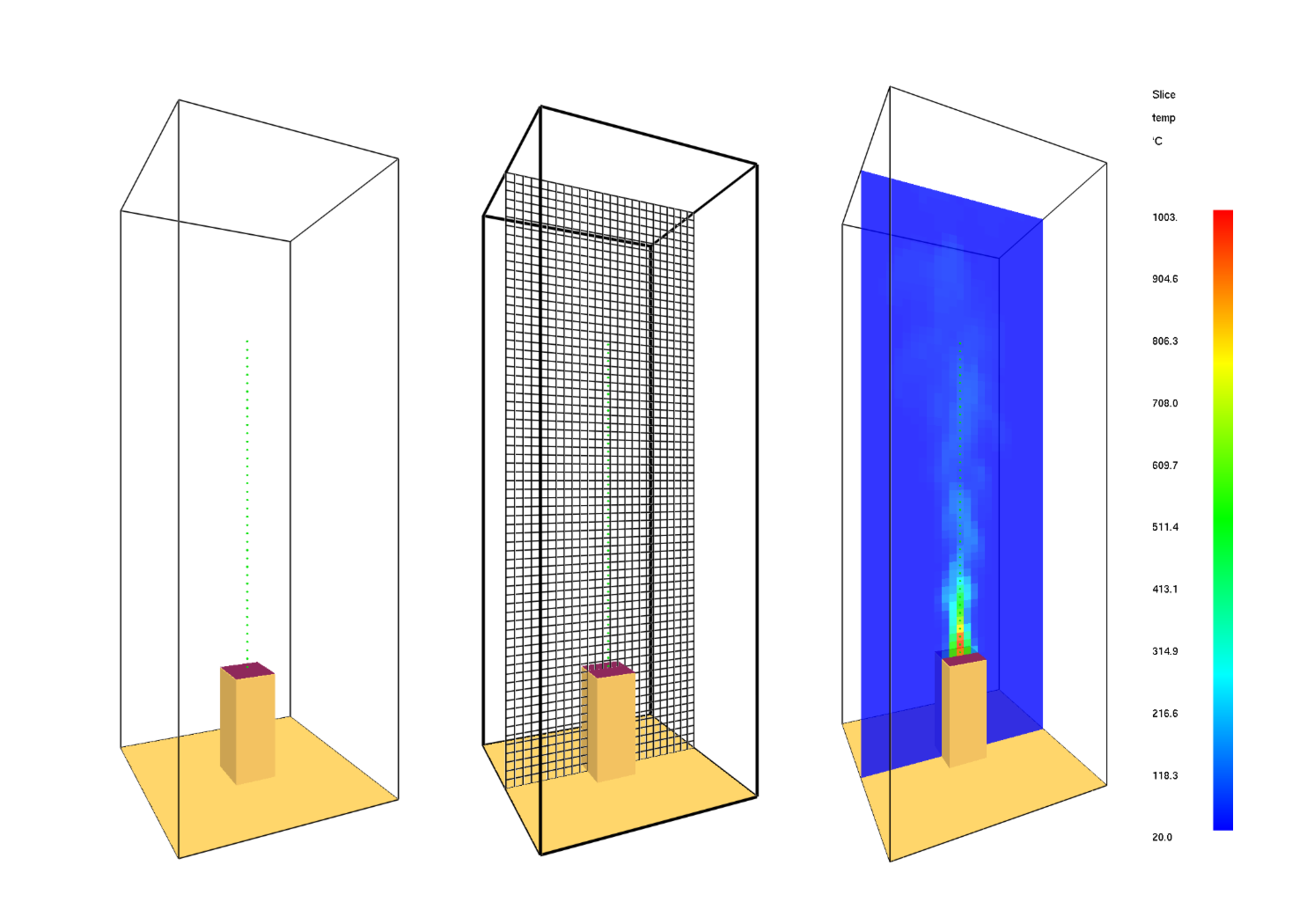
../../../_images/extra_task_diffusion_flame_01.png — Fig. 3.17 Visualization of the simulation setup in Smokeview.#

At total, five different simulations need to be run, one for each heat release rate indicated above.

Collecting and plotting the results

Once the simulations are finished, the data recorded by the devices (temperature and velocity) can be collected from the “devc.csv” output file. The goal is to present a log-log plot of the time-averaged output quantities against the hight above the burner, for the five values of heat release rates. Velocity and hight should be both normalised respectively by the scaling factors $\small\sf Q^{1/5}$ and $\small\sf Q^{2/5}$. The results obtained in the report are presented:

../../../_images/extra_task_McCaffreyVelocity.png — Fig. 3.18 Normalised velocity plotted against normalised hights above burner.#

../../../_images/extra_task_McCaffreyTemperature.png — Fig. 3.19 Temperature plotted against normalised hights above burner.#

Relevant insights for the solution of this task are presented in the Example: McCaffrey plume experiments.

Task II - Plume Formulas#

This task targets the computation of the plume temperature with analytical methods in order to subsequently validate the results of an numerical simulation. For more detailed information on the theory and application of the plume formulas, please refer to the literature, e.g. Enclosure Fire Dynamics by B. Karlsson and J. Quintiere [KQ99].

Heskestad

$\small\sf \Delta T $ indicates the temperature rise in the plume centerline axis above ambient temperature:

\[ \small\sf \Delta T = 9.1 \left(\frac{T_\infty}{g \cdot c_p^2 \cdot \rho_\infty^2} \right)^{1/3} \cdot \dot{Q}_c^{2/3} \cdot (z -z_0)^{-5/3} \]

where $\sf \dot{Q}_c$ is the convective heat release rate, $\small\sf T_\infty = 293~K$ is the ambient temperature, $\small\sf g = 9.81~ms^{-1}$ is the gravitational constant, $\small\sf \rho_\infty = 1.2 kg/m^3$ is the density of air at ambient temperature, $\small\sf c_p = 1.0~kJ/(kg K)$ is the specific heat capacity and z is the height above the fuel source in m.

The virtual origin $\small\sf z_0$ depends on the (equivalent) diameter D of the fire source and the total heat release rate and is given by:

\[\small\sf z_0 = 0.083 \cdot \dot{Q}^{2/5} - 1.02 \cdot D \]

The calculation of the plume temperature according to Heskestad is defined exclusively for the area above the flame. The flame height is calculated by the following expression:

\[\small\sf L = 0.235 \cdot \dot{Q}^{2/5} - 1.02 \cdot D \]

McCaffrey

$\small\sf \Delta T $ indicates the temperature rise in the plume centerline axis above ambient temperature:

\[\small\sf \Delta T = \left(\frac{\kappa}{0.9 \cdot \sqrt{2g}}\right)^2 \cdot \left(\frac{z}{\dot{Q}^{2/5}}\right)^{2\eta-1} \cdot T_\infty \]

where $\small\sf \dot{Q}$ is the total heat release rate, $\small\sf T_\infty = 293~K$ is the ambient temperature, $\small\sf g = 9.81~ms^{-1}$ is the gravitational constant, z is the height above the fuel source in m. The constants $\small\sf \eta$ and $\small\sf \kappa$ vary depending on the plume regions and can be obtained from the following table.

Region	$ \small\sf \frac{z}{\dot{Q}^{2/5}}$	$\small\sf \eta$	$\small\sf \kappa$
Continuous	< 0.08	1/2	$\small\sf 6.8~[m^{1/2}/s]$
Intermittent	0.08-0.2	0	$\small\sf 1.9~[m/(kW^{1/5}s)]$
Plume	> 0.2	-1/3	$\small\sf 1.1~[m^{4/4}/(kW^{1/3}s)]$

Task:

Calculate the temperatures of the plume within the respective application limits using the analytical approaches of the Heskestad and McCaffrey Plumes with a HRR of 1 MW at heights of $\small\sf z = 1~m, 2~m, 3~m, 4~m, 5~m, 6~m$. Assume that the radiative fraction of the plume is 20 % and $ \small\sf A_{fire}=1~m^2$ . Compare the results and discuss the reasons for the deviations.
Compare the results from the analytical calculations to the results of an FDS simulation using temperature devices. Smooth the output by a moving average to reduce noise. Refer to section 20.1 of the FDS User’s Guide for further information on how to place Devices in the computational domain.

Add the following lines to your FDS file to open the lateral and top boundaries of the sealed domain which provides a better depiction of the boundary conditions of the empirically determined plume formulas:
```
&VENT MB = 'XMIN' SURF_ID = 'OPEN' /
&VENT MB = 'XMAX' SURF_ID = 'OPEN' /
&VENT MB = 'YMIN' SURF_ID = 'OPEN' /
&VENT MB = 'YMAX' SURF_ID = 'OPEN' /
&VENT MB = 'ZMAX' SURF_ID = 'OPEN' /
```

Tip

To reduce noise, temperatures calculated with FDS can be smoothed using a simple moving average (SMA). The SMA of a time series $\small\sf x(t)$ is the sequence of arithmetic averages of $\small\sf n$ consecutive data points. $\small\sf m_{SMA}(t) = \frac{1}{n}\sum_{i=0}^{n-1}x(t-i)$

1. Solution:

Heskestad

Simplifying the plume formula into:

$\small\sf \Delta T = 9.1 \left(\frac{T_\infty}{g \cdot c_p^2 \cdot \rho_\infty^2} \right)^{1/3} \cdot \dot{Q}_c^{2/3} \cdot (z -z_0)^{-5/3} = 25 \left( \frac{\dot{Q}_c^{2/5}}{(z -z_0)}\right)^{5/3}$

The equivalent diameter:

$\small\sf D = \sqrt{\frac{4 \cdot A}{\pi}} = \sqrt{\frac{4 \cdot 1}{\pi}} \approx 1.13~m$

The virtual plume origin:

$\small\sf z_0 = 0.083 \cdot 1000^{2/5} - 1.02 \cdot 1.13 \approx 0.163~m$

The flame height:

$\small\sf L = 0.235 \cdot 1000^{2/5} - 1.02 \cdot 1.13 = 2.57~m$

The plume temperature at different heights:

$\small\sf z = 3.0 m:$ $\small\sf \Delta T = 25 \left( \frac{800^{2/5}}{(3 - 0.163)}\right)^{5/3} = 379~K$

$\small\sf z = 4.0 m:$ $\small\sf \Delta T = 25 \left( \frac{800^{2/5}}{(4 - 0.163)}\right)^{5/3} = 229~K$

$\small\sf z = 5.0 m:$ $\small\sf \Delta T = 25 \left( \frac{800^{2/5}}{(5 - 0.163)}\right)^{5/3} = 156~K$

$\small\sf z = 6.0 m:$ $\small\sf \Delta T = 25 \left( \frac{800^{2/5}}{(6 - 0.163)}\right)^{5/3} = 114~K$

McCaffrey

$\small\sf z = 1.0 m: \frac{z}{\dot{Q}^{2/5}} = \frac{1}{1000^{2/5}} = 0.063~|~0.063 < 0.08$ -> Continuous

$\small\sf z = 2.0 m: \frac{z}{\dot{Q}^{2/5}} = \frac{2.0}{1000^{2/5}} = 0.126~|~0.2 > 0.126 > 0.08$ -> Intermediate

$\small\sf z = 3.0 m: \frac{z}{\dot{Q}^{2/5}} = \frac{3.0}{1000^{2/5}} = 0.189~|~0.2 > 0.189 > 0.08$ -> Intermediate

$\small\sf z = 4.0 m: \frac{z}{\dot{Q}^{2/5}} = \frac{4.0}{1000^{2/5}} = 0.252~|~0.252 > 0.2$ -> Plume

$\small\sf z = 5.0 m: \frac{z}{\dot{Q}^{2/5}} = \frac{5.0}{1000^{2/5}} = 0.315~|~0.315 > 0.2$ -> Plume

$\small\sf z = 6.0 m: \frac{z}{\dot{Q}^{2/5}} = \frac{6.0}{1000^{2/5}} = 0.379~|~0.379 > 0.2$ -> Plume

The calculated temperatures and the respective auxiliary constants used can be found in the following table:

$\small\sf z [m]$	$\small\sf \frac{z}{\dot{Q}^{2/5}}[m/kW^{2/5}]$	$\small\sf \eta$	$\small\sf \kappa$	$\small\sf \Delta T [\circ C]$
1.0	0.063	1/2	$\small\sf 6.8~m^{1/2}/s$	852
2.0	0.126	0	$\small\sf 1.9~m/(kW^{1/5}s)$	528
3.0	0.189	0	$\small\sf 1.9~m/(kW^{1/5}s)$	352
4.0	0.252	-1/3	$\small\sf 1.1~m^{4/4}/(kW^{1/3}s)$	221
5.0	0.315	-1/3	$\small\sf 1.1~m^{4/4}/(kW^{1/3}s)$	152
6.0	0.379	-1/3	$\small\sf 1.1~m^{4/4}/(kW^{1/3}s)$	113

FDS Devices

2. Solution

../../../_images/pool_fire_1mw_open_temperatures_devc.svg — Fig. 3.20 Moving average of `TEMPERATURE` devices at heights 1.0, 2.0, 3.0, 4.0, 5.0 and 6.0 m smoothed over 100 datapoints.#

Task III – Time-dependent Heat Release Rate#

This task deals with the different possibilities to define the heat release rate (HRR) of a design fire and to model it in FDS. The total heat release $\small\sf \dot{Q}$ of a burning area $\small\sf A_{fire}$ depends on the heat release rate per unit area $\small\sf \dot{q}''$:

\[\small\sf \dot{Q} = {A_{Fire} \cdot \dot{q}''}\]

In FDS a burning area is defined by a VENT with a certain surface property that can be assigned by a SURF_ID. A fixed heat release rate per unit area can be set to a SURF by the attribute HRRPUA. Please refer to section 10.2.1 “Basics” of the FDS User’s Guide for further information.

Tip

Create an automation in Python or Excel that outputs the strings of the RAMP lines for the FDS input file.

Task:

Model the HRR progression for a radially spreading fire with a maximum power of 1 MW in FDS assuming a fixed burning area (task 1.1) and a radial propagation from the center of the burning area (task 1.2).
1. The HRR according to the ‘t-square’ model can be described by:
  
  \[\small\sf \dot Q = \alpha \cdot t^2\]
  
  where t is the burning time after ignition and $\small\sf \alpha$ is the fire growth factor.Assume a fast fire propagation by $\small\sf \alpha = 0.04689~kW/s^2$ and a constant heat release rate per unit area of $\small\sf \dot{q}'' = 0.25~MW/m^2$. The maximum burning area is $\small\sf A_{fire} = 1~m^2$. First calculate the time until the fire has spread to the entire area. This corresponds to the time at which the maximum HRR is reached. For simplicity, assume a perfect radial fire spread and a round fire area. Then model the temporal evolution of the HRR in FDS via a RAMP function (See section 20.6 “Controlling a Ramp” of the FDS User’s Guide ).
2. Model the fire propagation directly in FDS by defining the spread rate. The SPREAD attribute denotes a constant radial propagation speed from a specified point.
  
  Fig. 3.21 Fire propagation via FDS SPREAD attribute#
  
  For instructions on how to model a radial fire spread in FDS, please refer to the FDS User’s Guide Section 11.4.2 “Special Topic: A Radially-Spreading Fire”. The radial propagation speed v can be obtained from the fire area $\small\sf A_{Fire}$ and the corresponding burning period t.
  
  \[\small\sf v = \frac{\sqrt{A_{fire}/\pi}}{t}\]
3. Compare the HRR curves calculated by FDS with each other and discuss the limitations and inaccuracies associated with each approach.
Given is the fictional mass loss of a heptane fire. Calculate the heat release of the fire over the entire burning period with an assumed effective heat of combustion $\small\sf \Delta h_{c,eff} = 44,590~kJ / kg$. Model the HRR in FDS by using the RAMP function. Check if the simulated curve matches the prescribed HRR. The effective heat of combustion indicates the heat release per unit of weight of a material burned in combustion. For simplicity, assume that the averaged mass loss between two time steps applies to the end of each time interval. The mass loss caused by the burn-up can be described by the following time-dependent correlation:
```
time_index = [0, 25, 50, 75, 100, 125, 150, 175, 200, 225, 250, 275 ] # [s]
total_mass = [4000, 4000, 3600, 3040, 2880, 2400, 1800, 1120, 600, 160, 0, 0] # [g]
```

1. Solution

The burning period for the fire to reach the maximum heat release is:

\[ t = \frac{\dot{q}'' \cdot A_{Fire}}{\alpha} = \frac{250 \cdot 1}{0.04689} \approx 73~s \]

By setting the time and fraction parameters T and F, the RAMP function is obtained as follows:

&SURF ID = 'BURNER', HRRPUA = 250, RAMP_Q = 'fireramp', COLOR = 'RASPBERRY' /
&VENT XB = -0.5,0.5, -0.5,0.5, 0.0, 0.0, SURF_ID='BURNER' /
&RAMP ID='fireramp', T=0, F=0.00
.
.
.
&RAMP ID='fireramp', T=73, F=1.00

The spread rate corresponds to the propagation speed in m/s:

\[ \small\sf v = \frac{\sqrt{A_{fire}/\pi}}{t} = \frac{\sqrt{1/\pi}}{73} = 0.00773 m/s \]

Starting from the center of the vent, the radial propagation of the fire in FDS can be described as follows:

&SURF ID = 'BURNER', HRRPUA = 250, COLOR = 'RASPBERRY' /
&VENT XB = -0.5,0.5, -0.5,0.5, 0.0, 0.0, SURF_ID='BURNER', SPREAD_RATE = 0.00773 /

Show code cell content Hide code cell content

alpha = 0.04689
Qdot_max = 250
t = (Qdot_max / alpha)**(1/2)
print(t)
print(f"&SURF ID = 'BURNER', HRRPUA = {Qdot_max}, RAMP_Q = 'fireramp', COLOR = 'RASPBERRY' /")
for t in range(0, 74):
    Qdot = alpha * t **2
    
    print(f"&RAMP ID='fireramp', T={t}, F={Qdot / Qdot_max:.2f}")

73.01799238972059
&SURF ID = 'BURNER', HRRPUA = 250, RAMP_Q = 'fireramp', COLOR = 'RASPBERRY' /
&RAMP ID='fireramp', T=0, F=0.00
&RAMP ID='fireramp', T=1, F=0.00
&RAMP ID='fireramp', T=2, F=0.00
&RAMP ID='fireramp', T=3, F=0.00
&RAMP ID='fireramp', T=4, F=0.00
&RAMP ID='fireramp', T=5, F=0.00
&RAMP ID='fireramp', T=6, F=0.01
&RAMP ID='fireramp', T=7, F=0.01
&RAMP ID='fireramp', T=8, F=0.01
&RAMP ID='fireramp', T=9, F=0.02
&RAMP ID='fireramp', T=10, F=0.02
&RAMP ID='fireramp', T=11, F=0.02
&RAMP ID='fireramp', T=12, F=0.03
&RAMP ID='fireramp', T=13, F=0.03
&RAMP ID='fireramp', T=14, F=0.04
&RAMP ID='fireramp', T=15, F=0.04
&RAMP ID='fireramp', T=16, F=0.05
&RAMP ID='fireramp', T=17, F=0.05
&RAMP ID='fireramp', T=18, F=0.06
&RAMP ID='fireramp', T=19, F=0.07
&RAMP ID='fireramp', T=20, F=0.08
&RAMP ID='fireramp', T=21, F=0.08
&RAMP ID='fireramp', T=22, F=0.09
&RAMP ID='fireramp', T=23, F=0.10
&RAMP ID='fireramp', T=24, F=0.11
&RAMP ID='fireramp', T=25, F=0.12
&RAMP ID='fireramp', T=26, F=0.13
&RAMP ID='fireramp', T=27, F=0.14
&RAMP ID='fireramp', T=28, F=0.15
&RAMP ID='fireramp', T=29, F=0.16
&RAMP ID='fireramp', T=30, F=0.17
&RAMP ID='fireramp', T=31, F=0.18
&RAMP ID='fireramp', T=32, F=0.19
&RAMP ID='fireramp', T=33, F=0.20
&RAMP ID='fireramp', T=34, F=0.22
&RAMP ID='fireramp', T=35, F=0.23
&RAMP ID='fireramp', T=36, F=0.24
&RAMP ID='fireramp', T=37, F=0.26
&RAMP ID='fireramp', T=38, F=0.27
&RAMP ID='fireramp', T=39, F=0.29
&RAMP ID='fireramp', T=40, F=0.30
&RAMP ID='fireramp', T=41, F=0.32
&RAMP ID='fireramp', T=42, F=0.33
&RAMP ID='fireramp', T=43, F=0.35
&RAMP ID='fireramp', T=44, F=0.36
&RAMP ID='fireramp', T=45, F=0.38
&RAMP ID='fireramp', T=46, F=0.40
&RAMP ID='fireramp', T=47, F=0.41
&RAMP ID='fireramp', T=48, F=0.43
&RAMP ID='fireramp', T=49, F=0.45
&RAMP ID='fireramp', T=50, F=0.47
&RAMP ID='fireramp', T=51, F=0.49
&RAMP ID='fireramp', T=52, F=0.51
&RAMP ID='fireramp', T=53, F=0.53
&RAMP ID='fireramp', T=54, F=0.55
&RAMP ID='fireramp', T=55, F=0.57
&RAMP ID='fireramp', T=56, F=0.59
&RAMP ID='fireramp', T=57, F=0.61
&RAMP ID='fireramp', T=58, F=0.63
&RAMP ID='fireramp', T=59, F=0.65
&RAMP ID='fireramp', T=60, F=0.68
&RAMP ID='fireramp', T=61, F=0.70
&RAMP ID='fireramp', T=62, F=0.72
&RAMP ID='fireramp', T=63, F=0.74
&RAMP ID='fireramp', T=64, F=0.77
&RAMP ID='fireramp', T=65, F=0.79
&RAMP ID='fireramp', T=66, F=0.82
&RAMP ID='fireramp', T=67, F=0.84
&RAMP ID='fireramp', T=68, F=0.87
&RAMP ID='fireramp', T=69, F=0.89
&RAMP ID='fireramp', T=70, F=0.92
&RAMP ID='fireramp', T=71, F=0.95
&RAMP ID='fireramp', T=72, F=0.97
&RAMP ID='fireramp', T=73, F=1.00

../../../_images/pool_fire_10mw_sealed_hrr_spread.svg — Fig. 3.22 Simulated `HRR` generated by `RAMP` and `SPREAD` as a function of time.#

2. Solution

The HRR can be obtained from the mass loss $\small\sf \dot{m_{fuel}}$ by the following expression: $$\small\sf \dot{Q} = \Delta h_{c,eff} \dot{m_{fuel}}$$

The maximum

&SURF ID = 'BURNER', HRRPUA = 1212.85, RAMP_Q = 'fireramp', COLOR = 'RASPBERRY' /
&RAMP ID='fireramp', T=0, F=0.00 /
&RAMP ID='fireramp', T=25, F=0.15 /
&RAMP ID='fireramp', T=50, F=0.59 /
&RAMP ID='fireramp', T=75, F=0.68 /
&RAMP ID='fireramp', T=100, F=0.35 /
&RAMP ID='fireramp', T=125, F=0.59 /
&RAMP ID='fireramp', T=150, F=0.88 /
&RAMP ID='fireramp', T=175, F=1.00 /
&RAMP ID='fireramp', T=200, F=0.76 /
&RAMP ID='fireramp', T=225, F=0.65 /
&RAMP ID='fireramp', T=250, F=0.24 /
&RAMP ID='fireramp', T=275, F=0.00 /

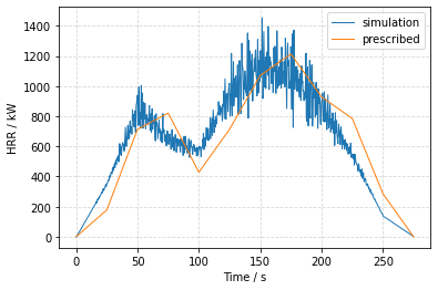
../../../_images/pool_fire_hrr_heptane_ramp.svg — Fig. 3.23 Prescribed and simulated `HRR` of n-heptane fire as a function of time. The heat release can be derived from the mass loss and the effective heat of combustion $\small\sf \Delta h_{c,eff}$.#

Task IV – Grid Convergence / HPC computing / Benchmarking#

This task deals with the monitoring of simulation parameters such as computation time and the convergence of numerical solutions.

Task:

Increase / decrease the grid resolution by factors of 0.4 and 2. Monitor the computing time by evaluating the .out file.
Extend the examination by refining the grid by a factor of 4 and 8, using resources of parallel computing. For this purpose subdivide the computational domain into several meshes.
Analyze the computation time for assigning multiple cores to a single OpenMP process. Split the computational domain into different meshes and assign individual MPI processes to each of them. Try to combine MPI and OpenMP and evaluate the increase in performance.
Check grid convergence for the respective resolutions of the domain based on temperature and velocity criteria

Solution:

../../../_images/pool_fire_benchmarking.svg — Fig. 3.24 Total computation time as a function of the total number of grid cells in the computational domain ( $\sf N_{cells}$ ) for different amount of openMP processes ($\sf N_{openMP}$).#

../../../_images/pool_fire_grid_convergence.svg — Fig. 3.25 Checking grid convergence for a device with quantity `TEMPERATURE` at XYZ (0, 0, 1). A grid size of 20 cm and below, which results in a total number of 31250 cells, does not show any significant change in temperature.#

Region	\( \small\sf \frac{z}{\dot{Q}^{2/5}}\)	\(\small\sf \eta\)	\(\small\sf \kappa\)
Continuous	< 0.08	1/2	\(\small\sf 6.8~[m^{1/2}/s]\)
Intermittent	0.08-0.2	0	\(\small\sf 1.9~[m/(kW^{1/5}s)]\)
Plume	> 0.2	-1/3	\(\small\sf 1.1~[m^{4/4}/(kW^{1/3}s)]\)

\(\small\sf z [m]\)	\(\small\sf \frac{z}{\dot{Q}^{2/5}}[m/kW^{2/5}]\)	\(\small\sf \eta\)	\(\small\sf \kappa\)	\(\small\sf \Delta T [\circ C]\)
1.0	0.063	1/2	\(\small\sf 6.8~m^{1/2}/s\)	852
2.0	0.126	0	\(\small\sf 1.9~m/(kW^{1/5}s)\)	528
3.0	0.189	0	\(\small\sf 1.9~m/(kW^{1/5}s)\)	352
4.0	0.252	-1/3	\(\small\sf 1.1~m^{4/4}/(kW^{1/3}s)\)	221
5.0	0.315	-1/3	\(\small\sf 1.1~m^{4/4}/(kW^{1/3}s)\)	152
6.0	0.379	-1/3	\(\small\sf 1.1~m^{4/4}/(kW^{1/3}s)\)	113

Example – Pool Fire

Contents

3.2. Example – Pool Fire#

Introduction#

Setup#

FDS Input File#

SMV Visualisation#

Analysis#

Task I – Basics#

Extra Task: Simulation of a purely buoyant diffusion flame#

Task II - Plume Formulas#

Task III – Time-dependent Heat Release Rate#

Task IV – Grid Convergence / HPC computing / Benchmarking#