2.1. Fluids

Overview

Fluid dynamics describes the movement of liquids or gases. The following aspects may be needed to be taken into account:

• compressibility

• boundary conditions, e.g. walls

• turbulence

• heat conduction

• chemical reactions

• multiple species and states of matter

• etc.

Fire safety science

In fire safety science, fluid dynamics plays an important role in the understanding of dynamical fire phenomena. Fluid dynamics must be considered e.g. during mixing processes, combustion, convective heat transfer or smoke spread in complex buildings.

Technical applications

A classical application example is the optimisation of transport vehicles to reduce the drag.

Fundamentals

In fluid dynamics, the following processes represent the most fundamental ones:

• Flow describes the movement of the medium. It is a vector field and describes the velocity of the fluid at every point in space and time: \(\mf \vv = \vv(x,t)\). The velocity components are denoted as \(\mf \vv = (v_x,v_y,v_z) = (u,v,w)\).

• Convection is the fluid intrinsic movement, i.e. due to buoyancy.

• Advection describes the transport of matter or properties (density, temperature, smoke) due to the flow. Convection is the advection of the velocity.

• Diffusion is a process that drives a balancing process to equilibrate differences in flow properties (velocity, temperature, smoke density).

Flow Quantities

Table 2.1 Flow quantities.

Name	Symbol	Unit	Type
density	\(\mf \rho\)	\(\mf kg/m^3\)	scalar field
velocity	\(\mf \vv\)	\(\mf m/s\)	vector field
vorticity	\(\mf \vec{\omega} = \nabla \times \vv\)	\(\mf 1/s\)	vector field
momentum density	\(\mf \vu = \rho\vv\)	\(\mf kg/(m^2~s)\)	vector field
pressure	\(\mf p\)	\(\mf Pa = kg/(m~s^2)\)	scalar field
temperature	\(\mf T\)	\(\mf K\)	scalar field
specific enthalpy	\(\mf h = \int_{T_0}^T c_p(T')\ dT' + \Delta h_f^0\)	\(\mf J/kg = m^2/s^2\)	scalar field

Where \(\mf c_p(T)\) is the heat capacity at temperature \(\mf T\) and \(\mf \Delta h_f^0\) is the heat of formation.

Speed of Sound

In fluids and solids, information (flow changes, perturbations) propagates with a finite speed: the speed of sound. Sound waves are longitudinal compression waves. Typical travel speeds are \(\mf 343~m/s\) in air, \(\mf 1484~m/s\) in water and \(\mf 5120~m/s\) in steel. In general, the speed of sound \(\mf c_s\) in an ideal gas is given by:

(2.1)\[ \mf c_s = \sqrt{\frac{\gamma k_B T}{m}} \]

where \(\mf \gamma\) is the heat capacity ratio \(\mf \gamma=c_P/c_V\), \(\mf k_B\) is the Boltzmann constant (\(\mf \sim\!1.381\cdot 10^{−23}~J/K\)), T the gas temperature, and \(\mf m\) the mass of a single gas molecule. In general, for a given gas species, the speed of sound depends only on the temperature. For dry air, it can be approximated as:

(2.2)\[ \mf c_{s, air} =(331.3+0.606\cdot \Theta) m/s \]

where \(\mf \Theta\) is the air temperature in \(\mf ^\circ C\).

Equation of State

For an ideal, or perfect, gas the state can usually be described in terms of two thermodynamic variables (\(\mf n\), \(\mf\rho\), \(\mf p\), \(\mf e\), \(\mf T\), \(\mf V\), \(\mf m\), \(\mf h\)). Following the combination of Boyle’s and Charles’ laws in a thermodynamical equilibrium, the equation of state follows as:

(2.3)\[ \mf pV = nRT \]

where \(\mf R = 8.314~J/(mol~K)\) is the universal gas constant and \(\mf n\) is the number of particles. Reactive flows are mostly a compound of a number of different species. Thus, the equation of state for a system in equilibrium with \(\mf N\) species becomes

\[ \mf p = f(V, T, n_1 , \dots , n_N)\quad . \]

Dalton’s law of partial pressures \(\mf p_i\) allows to formulate the total pressure

\[ \mf p = \sum_{i=1}^N p_i = \frac{1}{V} \sum_{i=1}^N n_i R T\quad . \]

Characterisation of Flows

Flows of fluids (liquids and gases) follow the same principal characteristics. In the following, there will be no difference in liquid or gas flows. They will only differ in material properties. Examples for a fluid flow:

Fig. 2.1 Von Kármán vortex street observed in nature. Soruce: Wikkimedia Commons.

Fig. 2.2 Von Kármán vortex street in a lab. Soruce: Wikkimedia Commons.

Compressible Flows

For flows with velocities much slower (\(\mf \ll c_s\)) than the speed of sound, pressure variations are very small and the fluid can be considered incompressible. the sound waves are infinitely fast on the scale of the involved processes. Thus, all changes in density are quickly balanced. For modelling, this is important because the pressure and density equations can be decoupled due to the assumed incompressibility. Objects traveling with a speed of at least \(\mf 0.3c_s\) start to introduce fluctuations in density. Flow patterns of super-sonic phenomena (explosions/detonations, supersonic airplanes, space craft re-entry) and the corresponding engineering approaches are completely different to those in case of sub-sonic flows.

Note: Temperature changes, like in a fire, lead to density changes and therefore to so called weakly compressible flows.

Fig. 2.3 Incompressilbe flow around a model car. Source: Wikkimedia Commons.

Fig. 2.4 Super-sonic airplane model in a tunnel with at approximately \(\mf 3.5 c\). Source: Wikkimedia Commons.

Turbulent Flows

Depending on how smooth (continuous) a flow is, one can distinguish between laminar and turbulent flows. Flows related to fires are typically turbulent.

Fig. 2.5 Flow around an airfoil with a flow separation. Soruce: Wikkimedia Commons.

Material Parameters

The following material properties are of fundamental interest:

• density \(\mf\rho\) is the mass per given volume

  • air at \(\mf 20~^\circ C\) : \(\mf\rho = 1.205~kg/m^3\)

  • air at \(\mf 200~^\circ C\): \(\mf\rho = 0.746~kg/m^3\)

• dynamic viscosity \(\mf\mu\) characterises the capability of a flow to balance differences in velocity

  • air at \(\mf 20~^\circ C\) : \(\mf\mu = 1.836\cdot 10^{-5}~kg\,m / s\)

  • air at \(\mf 200~^\circ C\): \(\mf\mu = 2.623\cdot 10^{-5}~kg\,m / s\)

• thermal conductivity \(\mf k\) is equivalent to \(\mf\mu\), but for the temperature of a fluid

  • air at \(\mf 20~^\circ C\) : \(\mf k = 0.0257~W\,m / K\)

  • air at \(\mf 200~^\circ C\): \(\mf k = 0.0386~W\,m / K\)

• heat capacity \(c_p\) describes the change in temperature, due to adding or extracting heat at a constant pressure

  • air at \(\mf 20~^\circ C\) : \(\mf c_p = 1.005~kJ\,kg / K\)

  • air at \(\mf 200~^\circ C\): \(\mf c_p = 1.026~kJ\,kg / K\)

Further data for many properties of air (and other materials) can be found at Engineering ToolBox (air properties).

Example quantity: viscosity

Simply speaking, viscosity describes how moving fluid elements, e.g. layers, influence the neighbouring elements. It describes the friction forces between relatively moving fluid elements.

For example, honey has a high viscosity: it flows only slowly down a spoon. The outer ”honey elements” are strongly coupled to the inner – not free – elements.

Fig. 2.6 Honey running down a spoon. Soruce: Wikkimedia Commons.

In a simple two dimensional setup, with a stationary wall and a moving wall, see Fig. 2.7, the dynamic viscosity describes the relation of the forces on the walls and the velocity gradient. If the velocity gradient \(\mf u/y\) is constant, this results in the following friction force per area:

(2.4)\[ \mf \frac{F}{A} = \mu \cdot \frac{u}{y} \]

Fig. 2.7 Visualisation of the viscosity concepte. Soruce: Wikkimedia Commons.

Relation (2.4) is the definition of the dynamic viscosity \(\mf \mu\). Yet, in some cases the kinematic viscosity \(\mf \nu\) (or momentum diffusivity) is a more convenient quantity. It is given by the ratio of the dynamic viscosity and the density

(2.5)\[ \mf \nu = \frac{\mu}{\rho} \quad . \]

Fluids for which viscosity does not depend on the stress state are called Newtonian fluids, all gases are Newtonian fluids. However, there exist also non-Newtonian fluids, like blood, tomato ketchup and water mixed with corn starch.

Dimensionless numbers

Many flow phenomena and types may be characterised by dimensionless numbers. It is assumed, that flows with similar characteristics are comparable, although for example the spatial scales are different. Some of the commonly used dimensionless numbers are:

• Mach number \(\mf Ma\)

• Reynolds number \(\mf Re\)

• Grashof number \(\mf Gr\)

• Prandtl number \(\mf Pr\)

• Archimedes number \(\mf Ar\)

• Richardson number \(\mf Ri\)

• Nusselt number \(\mf Nu\)

Mach number

The Mach number is defined as the relation of a velocity to the speed of sound, i.e.

(2.6)\[ \mf Ma = \frac{v}{c_s} \]

This number characterises the compressibility of a flow:

• \(\mf Ma \rightarrow 0\): fully incompressible

• \(\mf Ma \lesssim 0.3\): incompressible

• \(\mf Ma \gtrsim 0.3\): compressible

The limit \(\mf Ma \rightarrow 0\) may be also interpreted as \(\mf c \rightarrow \infty\).

Reynolds number

The Reynolds number relates convection to diffusion:

\[ \mf Re = \frac{\rho v L}{\mu} \]

Here, \(\mf L\) denotes a characteristic length, in the case of a pipe flow, this would be the pipe diameter. The Reynolds number can be used to distinguish laminar from turbulent flows, i.e. a very high \(\mf Re\) represents turbulent flows. In a pipe flow, the characteristic transition number is about \(\mf Re \approx 4000\). This number is a classical example for scaling. Flow phenomena having the same Reynolds number will behave the same way; this can be shown by normalisation of the flow equations.

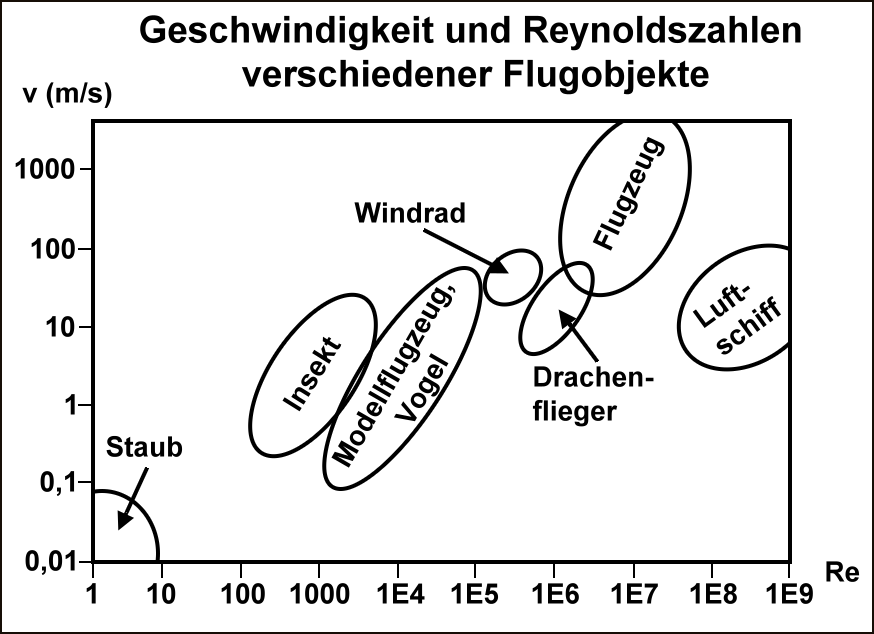
Fig. 2.8 Velocity and Reynolds numbers for some flying objects (in German). (Staub:Dust, Insekt:Insect, Modellflugzeug/Vogel:Aeroplane model/Bird, Windrad:Windmill, Drachenflieger:Hang glider, Flugzeug:Aeroplane, Luftschiff:Airship) Source: Wikkimedia Commons.

Fluid Equations

Conservation laws

Fluid dynamics is based on the following three physical conservation laws:

• mass conservation

• momentum conservation

• energy conservation

From these laws the basic fluid flow equations may be derived:

• continuity equation

• equation of motion

• energy equation

In general, beside these equations a closure is needed, for example via an equation of state. In many cases the ideal gas law can be used.

Conservation of mass

The conservation of mass predicts, that the total mass of a control volume only changes if there is a net flow (non balanced in and out flow) across the boundaries. Incompressible flows have always zero net flows.

In fire simulations, multiple species have to be considered (e.g. oxygen, fuel and carbon dioxide). Their masses are individually conserved. However, they are strongly coupled to each other via source terms. E.g. during combustion, oxygen and fuel are consumed to produce carbon dioxide.

Conservation of momentum

The momentum of a fluid element changes only due to:

• momentum advection

• gradients of pressure

• diffusion and stresses, i.e. due to finite viscosity

• external forces, e.g. gravitation, water droplets

In turbulent simulations, the diffusion is of special interest. This is the phenomenon that must be covered by turbulence models.

Conservation of energy

Changes in energy of a control volume are due to:

• energy advection

• heat conduction

• heating and cooling processes, e.g. radiation, friction, combustion

In combination with the conservation of energy, an equation of state is needed to determine the gas temperature.

Partial Differential Equations

Partial differential equations (PDE) are one of the most powerful tools in science and engineering. Most technical, mathematical, physical, chemical and even biological models are based on differential equations. The solutions of differential equations may describe:

• gas flows and combustion processes

• heat distribution in solids

• oscillation of a pendulum

• propagation of light or water waves

• interaction of two species (predator and pray)

Types of PDEs

The general structure of a PDE for \(\mf\phi = \phi(x,y)\) is given by

\[ \mf a\partial_{xx}\phi + b\partial_{xy}\phi + c\partial_{yy}\phi + d\partial_x\phi + e\partial_y\phi + f\phi = 0 \]

where all coefficients (\(\mf a,\dots,f\)) are dependent on \(\mf x\) and \(\mf y\), e.g. \(\mf a = a(x,y)\).

The coefficients determine the character of the PDE:

\[ \mf D(x,y) = a(x,y)\cdot c(x,y) - \left(\frac{b(x,y)}{2}\right)^2 \]

• \(\mf D \gt 0\): elliptic, e.g. Laplace equation

• \(\mf D = 0\): parabolic, e.g. heat equation

• \(\mf D \lt 0\): hyperbolic, e.g. wave equation

Note: The type may dependent on varying material parameters or/and the position, here \(\mf (x,y)\).

Field Operators

The two most common mathematical operators used in fluid dynamics are the partial derivative and the Nabla operator.

The partial derivative describes the change of a field in a given space or time direction. The change of a velocity field \(\mf \vv(x,y,z,t)\) with respect to the time is:

\[ \mf \frac{\partial \vec{v}(x,y,z,t)}{\partial t} \quad \mbox{or short}\quad \partial_t \vec{v}(x,y,z,t) \]

The Nabla operator \(\mf \nabla\) is used to represent the Laplace, gradient, divergence and rotation operations.

\[ \mf \nabla = \left( \partial_x, \partial_y, \partial_z \right) \]

\[\begin{split} \mf \Delta(\rho) = \nabla^2\rho \\ \mf grad(\rho) = \nabla\rho \\ \mf div(\vv) = \nabla\cdot\vv \\ \mf rot(\vv) = \nabla\times\vv \end{split}\]

The convective derivative combines both operators. It represents the total change of a value due to local intrinsic changes and due to advection. The change in a scalar value \(\mf \phi(x,y,z,t)\) may therefore be written as

\[ \mf \frac{d\phi}{dt} = \partial_t \phi + \vv\cdot(\nabla\phi) \]

The first term (\(\mf \partial_t \phi\)) represents intrinsic changes and the second one (\(\mf\vv\cdot(\nabla\phi)\)) describes the changes due to the advection in the velocity field \(\mf\vv\).

Continuity Equation

The continuity equation for a single species flow is

(2.7)\[ \mf \frac{d\rho}{dt} = \underbrace{-\rho\nabla\cdot\vec{v}}_{A} \]

• \(\mf A\): net flow flux of mass

Taking into account the convective derivative, the commonly used formulation may be derived as

(2.8)\[ \mf \partial_t \rho = -\nabla\cdot(\rho\vec{v})\quad . \]

Equation of motion

Taking into account the conservation of momentum, the following simple form of the equation of motion may be formulated

(2.9)\[ \mf \partial_t \rho\vec{v} + \nabla\cdot(\rho\vec{v}\vec{v}) = \underbrace{-\nabla p}_{A} + \underbrace{\mu\nabla^2\vec{v}}_{B} + \underbrace{\vec{f}}_{C} \]

• \(\mf A\): force due to pressure gradients

• \(\mf B\): molecular diffusion

• \(\mf C\): external forces, e.g. gravity

These equation is commonly known as the Navier-Stokes equation.

Energy equation

The equation for the energy \(E = e + \frac{1}{2}\vv^2\) is given by

(2.10)\[ \mf \partial_t (\rho E) + \nabla\cdot(\vec{v}\rho E) = \underbrace{-\nabla\cdot(\vec{v}p)}_{A} + \underbrace{\nabla\cdot(\mu\vec{v}\nabla\vec{v})}_{B} + \underbrace{\nabla\cdot(k\nabla T)}_{C}+ \underbrace{\vec{v}\cdot\vec{f}}_{D}+\underbrace{\dot{Q_s}}_{E} \]

• \(\mf A\): work done on the fluid due to pressure gradients

• \(\mf B\): work done by viscosity

• \(\mf C\): heat conduction

• \(\mf D\): work done by external forces

• \(\mf E\): heat sources and sinks

Note: Sometimes a formulation in terms of enthalpy is preferred. This is the case for the equations solved by FDS.

Incompressible equations

If the flow is incompressible and assumed to be isothermal, the remaining equations to be solved are:

\[\begin{split} \mf \partial_t \rho\vec{v} + \nabla\cdot(\rho\vec{v}\vec{v}) = -\nabla p + \mu\nabla^2\vec{v} + \vec{f} \\ \mf \nabla^2 p = - \nabla\cdot\left(\nabla\cdot(\rho\vec{v}\vec{v})\right) + \nabla \cdot \vec{f} \end{split}\]

Weakly compressible regime

In fully incompressible flows the pressure instantly balances all divergences and keeps therefore the density constant.

In the compressible regime, the ideal gas law provides the linkage between the energy conservation and the conservation of mass and momentum.

For low speed flows, like in fires, but with substantial temperature variations the density may change. This is not due to pressure variations, as the pressure remains relatively unperturbed. This is the so called weakly compressible regime.

Here the equation of state is used with a fixed ambient pressure \(\mf p_0\) to determine the density:

\[ \mf \rho = \frac{p_0 M}{R T} \]

with \(\mf M\) being the molecular mass of the volume of interest.

Boundary Conditions

Besides the fluid equations, the boundary conditions are an other important aspect. In many applications, the impact of boundary conditions is crucial and a proper treatment of those essential.

In general there exist a few types of boundary conditions:

• Dirichlet: explicit values are prescribed

  \[ \mf u=u_0\quad v=w=0 \]

• Neumann: normal derivative is prescribed

  \[ \mf \partial_n u = n_0\quad \partial_n v = \partial_n w = 0 \]

• symmetric: derivatives are adopted to preserve a prescribed symmetry

• periodic: values at the facing boundaries are kept equal

Some explicit examples for boundary conditions used commonly in fluid dynamics:

• no-slip at solid wall

  \[ \mf u = v = w = 0 \quad \mbox{at the wall} \]

• gas inlet

  \[ \mf u = u_0\quad v=w=0 \quad \mbox{at the inflow} \]

• gas outflow

  \[ \mf \partial_n u = \partial_n v = \partial_n w = 0\quad \mbox{at the outflow} \]

• constant wall temperature

  \[ \mf T = T_w \]

• wall with changing temperature, but fixed wall heat flux

  \[ \mf q_w = k \partial_n T\quad \mbox{at the wall} \]

• adiabatic

  \[ \mf k\partial_n T = 0 \quad \mbox{at the wall} \]

Fig. 2.9 Example for a boundary setup for a open plume.

Fig. 2.10 Example for a boundary setup for a simple compartment.