Fundamentals

3.1. Fundamentals#

In fire safety engineering compartment fires are an important topic. The development of a fire in a compartment determines the energy release and the spread of smoke through a building. This has direct on the safety of the occupants and how effective the fire brigade can deal with the fire. A good overview on modelling principles of compartment fires is given in the book “Enclosure Fire Dynamics” by Karlsson and Quinitere [KQ99]. We take some of the aspect described in this book and discuss them here in context of the lecture. The simulations themselves are built around some experiments that are fundamental to the field of fire safety engineering.

At first, we look into plume models and experiment data from McCaffrey [McC79], which are described in the report about “Purely Buoyant Diffusion Flames”. These plume experiments and respective models are a good starting point to modelling compartment fires. Using gas burners at different locations, Steckler et al. performed a number of experiments in a regular-sized compartment [SQR82] (\(\mf 2.8~m \times 2.8~m \times 2.18~m\)). The results are provided in the report “Flow Induced by Fire in a Compartment”.

This brief introduction into the fluid dynamics in a compartment fire is based on a characteristic setup and simulations carried out.

../../../_images/Steckler02.png

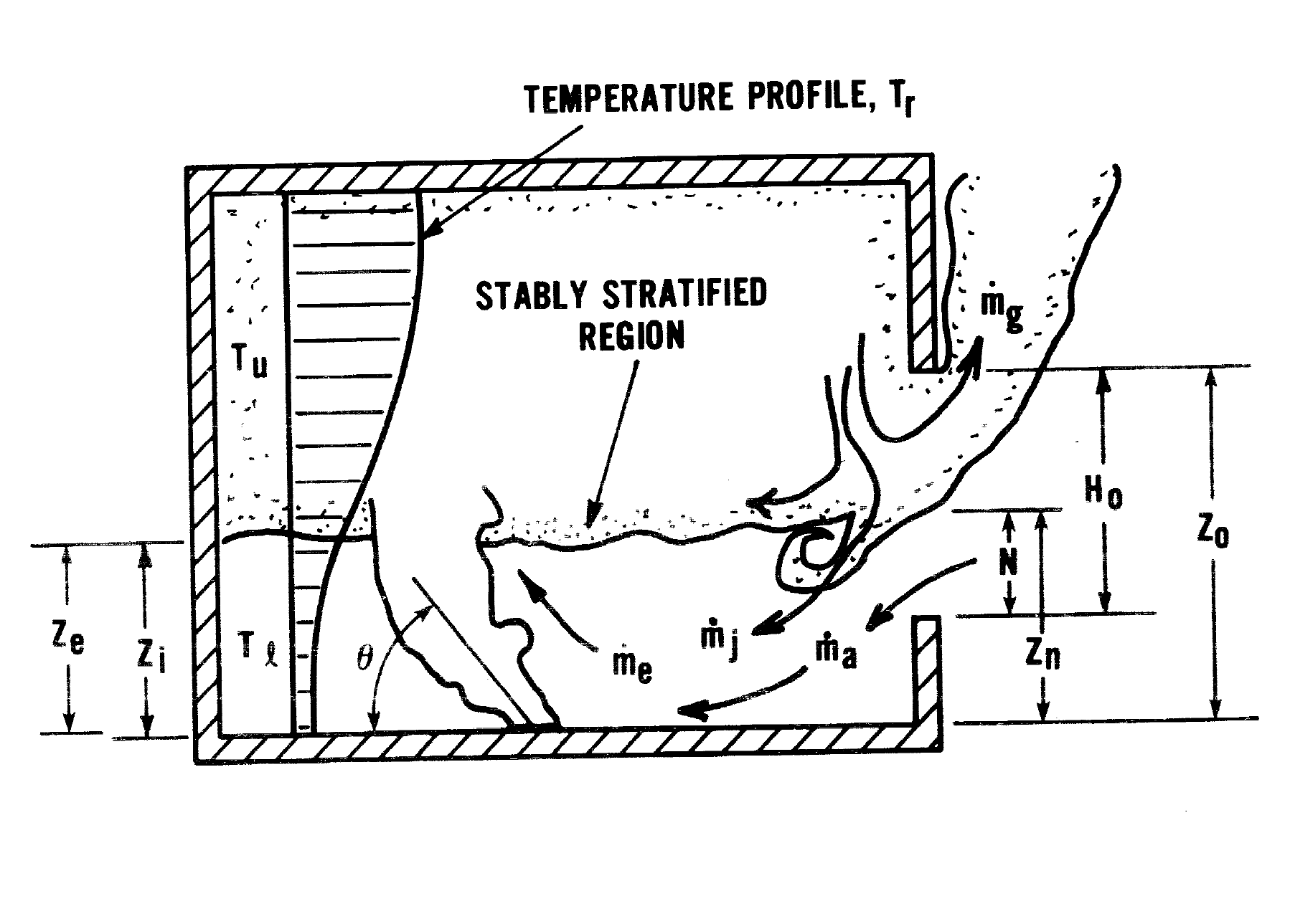
Fig. 3.1 Overview over the experimental setup used by Steckler et al. [SQR82].#

../../../_images/Steckler01.png

Fig. 3.2 Overview over the experimental setup used by Steckler et al. [SQR82].#

Setup#

The compartment has an extension of

\[ \mf I_{compartment} = [0.20~m, 2.70~m] \times [-1.40~m, 1.40~m] \times [0.05~m, 2.00~m] \]

and is embeded in a computational domain of

\[ \mf I_{domain} = [0.00~m, 4.80~m] \times [-1.80~m, 1.80~m] \times [0.00~m, 3.00~m] \quad . \]

The compartment is build out of individual obstacles, creating the walls, the floor and the ceiling. One of the walls contains an opening, see Fig. 3.3. The domain boundaries are defined as open boundaries.

../../../_images/compartment_fire_setup_01.png

Fig. 3.3 Setup for the compartment fire example. There is only a single opening, i.e. the door. The surface with a predefined heat release rate is indicated in red.#

The heat release rate is defined as a constant value of \(\mf 10~kW\) and the patch emitting the fuel has a surface temperature of \(\mf 100~^\circ C\).

For demonstration purposes, all quantities are visualised in the symmetry plane at \(\mf y=0\), see Fig. 3.4.

../../../_images/compartment_fire_slcf_temp_01.png

Fig. 3.4 Temperature field in the \(\mf y=0~m\) plane.#

Pressure#

Thermal expansion and differences in gas densities lead to pressure differences. These in turn are driving the gas flow in and out of the compartment. One can compare the pressuere differences inside and outside of a compartment, as well as changes with height. During different phases of a developing fire the pressure profiles change. In the very early phase it is considerd that there is mostly overpressure inside the room with respect to outside.

../../../_images/InitialFire.png

Fig. 3.5 Pressure profile in a compartment during the initial stage of a fire.#

When the fire developes a bit further a more pronounced pressure profile is generated. The height where the two graphs cross is considered the location of the “neutral plane” that spans the compartment. This is also highlighted in the plots further down, with the pressure slices. In the figure shown, it can be seen that the pressure inside the room starts out lower than outside. They run parallel for some distance and then the pressure inside increases notably. Around the bend, below the neutral plane, is typically the height of a relatively stable interface between the cold and hot gas layers. These observations form the basis for the zone models.

../../../_images/IntermediateFire.png

Fig. 3.6 Pressure profile in a compartment in an intermediate stage of a fire.#

The further the fire in a compartment can develop, the further the height of the cold gas layer drops. At some point there are no gas layers left to speak of and the room is considered fully envolved in the fire. Furthermore, it is visible that parts of the smoke get mixed into the air that flows into the compartment. Thus, over time the relatively smoke free lower layer get more and more enriched with smoke.

../../../_images/DevelopedFire.png

Fig. 3.7 Pressure profile in a compartment a a developed stage of a fire.#

list_q = ['PRESSURE', 'BACKGROUND PRESSURE']

it = sim.slices[0].get_nearest_timestep(250)

for q in list_q:
    slice = sim.slices.filter_by_quantity(q)[0]
    
#     print(slice)
    ### fds / fdsreader BUG workaround BEGIN
    ### Issue due to SLCF located at MESH boundary
    to_del = []
    for s in slice:
        if s.extent._extents[1][0] > 0:
            to_del.append(s.mesh)
    for m in to_del:
        del slice._subslices[m]
        
    extent = (slice.extent[0][0], slice.extent[0][1], 
              slice.extent[2][0], slice.extent[2][1])
#     print(extent)
    ### fds / fdsreader BUG workaround END
    
    slice_data = slice.to_global()
    
    if np.min(slice_data[it]) < 0:
        v_abs_max = np.max(np.abs(slice_data[it]))
        vmin = -v_abs_max
        vmax = v_abs_max
    else:
        vmin = np.min(slice_data[it])
        vmax = np.max(slice_data[it])
    
    plt.imshow(slice_data[it].T,
               vmin = vmin, vmax = vmax,
               origin='lower', 
               extent=extent,
               cmap='seismic')
    q = slice.quantity.quantity
    u = slice.quantity.unit
    plt.colorbar(label=f"{q} / {u}")
    plt.show()
---------------------------------------------------------------------------
NameError                                 Traceback (most recent call last)
Input In [1], in <cell line: 3>()
      1 list_q = ['PRESSURE', 'BACKGROUND PRESSURE']
----> 3 it = sim.slices[0].get_nearest_timestep(250)
      5 for q in list_q:
      6     slice = sim.slices.filter_by_quantity(q)[0]

NameError: name 'sim' is not defined

Flow#

import numpy as np
import matplotlib.pyplot as plt
import fdsreader

plt.rcParams['figure.dpi'] = 150
path_to_data = '../../../../data/compartment/pressure_01/rundir/'

sim = fdsreader.Simulation(path_to_data)
list_q = ['U-VELOCITY', 'V-VELOCITY', 'W-VELOCITY']
it = sim.slices[0].get_nearest_timestep(250)
for q in list_q:
    slice = sim.slices.filter_by_quantity(q)[0]
    
    print(slice)
    ### fds / fdsreader BUG workaround BEGIN
    ### Issue due to SLCF located at MESH boundary
    to_del = []
    for s in slice:
        if s.extent._extents[1][0] > 0:
            to_del.append(s.mesh)
    for m in to_del:
        del slice._subslices[m]
        
    extent = (slice.extent[0][0], slice.extent[0][1], 
              slice.extent[2][0], slice.extent[2][1])
#     print(extent)
    ### fds / fdsreader BUG workaround END
    
    slice_data = slice.to_global()
    
    v_abs_max = np.max(np.abs(slice_data[it]))
    
    plt.imshow(slice_data[it].T,
               vmin = -v_abs_max, vmax = v_abs_max,
               origin='lower', 
               extent=extent,
               cmap='seismic')
    q = slice.quantity.quantity
    u = slice.quantity.unit
    plt.colorbar(label=f"{q} / {u}")
    plt.show()
Slice([3D] cell_centered=True, extent=Extent([0.00, 4.80] x [0.00, 0.05] x [0.00, 3.00]))
../../../_images/bfd214d5f309f4e701b50a48b9e864c93b733eccabf7be19e7806652cd3aef6b.png
Slice([3D] cell_centered=True, extent=Extent([0.00, 4.80] x [0.00, 0.05] x [0.00, 3.00]))
../../../_images/8b66ec81ea1eb650a8bff3d0bb52cacdea98e706abfed953d381c88e49206362.png
Slice([3D] cell_centered=True, extent=Extent([0.00, 4.80] x [0.00, 0.05] x [0.00, 3.00]))
../../../_images/24dbde025d60ea230dcb5e770dbf7a026327092cd18a092dd74102c707d1c576.png
u_slice = sim.slices.filter_by_quantity('U-VELOCITY')[0]
slice_data = u_slice.to_global()
x0 = 2.7
ix = u_slice.get_nearest_index('x', x0)
print(f'Index in x-direction next to x={x0} is {ix}.')

z0 = 1.5
iy = u_slice.get_nearest_index('y', z0)
print(f'Index in z-direction next to z={z0} is {iy}.')
Index in x-direction next to x=2.7 is 54.
Index in z-direction next to z=1.5 is 35.
instant_values = slice_data[:, ix, iy]
n_a = 51
average_values = np.convolve(instant_values, np.ones(n_a)/n_a, mode='valid')
plt.plot(u_slice.times, instant_values, '.', color='grey', alpha=0.5, label='instanteneous values')
plt.plot(u_slice.times[n_a//2:-(n_a//2)], average_values, label='moving average')
plt.xlabel('Time / s')
plt.ylabel('Velocity Component $\sf v_x$ / m/s')
plt.grid()
plt.legend()
plt.title(f'Values at position (x,z)=({x0} m, {z0} m)');
../../../_images/0c8f5275b4628d7caa07c9b6b503e78e4103b3cee52a7b4c7558a7592c92d37f.png
z_max = 2.0
iz_max = u_slice.get_nearest_index('y', z_max) 

### TODO: quick solution, needs fix
h = np.arange(0, z_max, 0.05)

list_t = [10, 25, 50, 100, 250]

for t in list_t:
    it = sim.slices[0].get_nearest_timestep(t)
    plt.plot(slice_data[it, ix, 0:iz_max+5], h, label=f't={t}')

plt.xlabel('Velocity Component $\sf v_x$ / m/s')
plt.ylabel('Height / m')
plt.grid()
plt.legend()
<matplotlib.legend.Legend at 0x118679d90>
../../../_images/9b1dc99ad0980724c3a284f6f0a738d734425532dc368cac9980caefa8014054.png

Other Quantities#

list_q = ['TEMPERATURE', 'DENSITY', 'KOLMOGOROV LENGTH SCALE', 'SUBGRID KINETIC ENERGY', 'VORTICITY Y']
it = sim.slices[0].get_nearest_timestep(250)
for q in list_q:
    slice = sim.slices.filter_by_quantity(q)[0]
    
#     print(slice)
    ### fds / fdsreader BUG workaround BEGIN
    ### Issue due to SLCF located at MESH boundary
    to_del = []
    for s in slice:
        if s.extent._extents[1][0] > 0:
            to_del.append(s.mesh)
    for m in to_del:
        del slice._subslices[m]
        
    extent = (slice.extent[0][0], slice.extent[0][1], 
              slice.extent[2][0], slice.extent[2][1])
#     print(extent)
    ### fds / fdsreader BUG workaround END
    
    slice_data = slice.to_global()
    
    if np.min(slice_data[it]) < 0:
        v_abs_max = np.max(np.abs(slice_data[it]))
        vmin = -v_abs_max
        vmax = v_abs_max
        cmap='seismic'
    else:
        vmin = np.min(slice_data[it])
        vmax = np.max(slice_data[it])
        cmap='viridis'
    
    plt.imshow(slice_data[it].T,
               vmin = vmin, vmax = vmax,
               origin='lower', 
               extent=extent,
               cmap=cmap)
    q = slice.quantity.quantity
    u = slice.quantity.unit
    plt.colorbar(label=f"{q} / {u}")
    plt.show()
../../../_images/880309353ed966f048f1f7dd0ab4fa9bae8f79085024695ef260015822a3c612.png ../../../_images/4505f242759a323dd313d971509f13edee25f664db68090a7eb02c7182aa867a.png ../../../_images/f831ec037bf12d17b0bf92e0311bf7efe3aa1401b5626af730ed8c5f28b9aa8f.png ../../../_images/60b889823e090e4a33600599441c2a37d10cd5e3e58d77d67463786464ad679a.png ../../../_images/ab9979f63125e3591dc68eb7b64d564e88f1bd66c348970df193fd987845dc71.png