5.2. Modelling

Conserved Scalar Formulation

A simple combustion modelling approach is the assumption that chemical processes are infinitely fast, the so called mixed-is-burnt model. It is assumed, that the instantaneous thermostatic state is related to a scalar quantity known as mixture fraction \(\mf f =f(\vec{x},t)\). It is an artificial quantity that describes the mixing of species and varies in space in time. The individual species concentrations are derived from the mixture fraction.

Given a reaction volume, with an inflow of two (representative) species, e.g. fuel \(\mf Y_F\) and air \(\mf Y_A\), and an outflow of a mixture \(\mf Y_M\), the mixture fraction \(\mf f\) is defined as

\[ \mf f Y_F + (1-f)Y_A = Y_M \quad \Rightarrow \quad f=\frac{Y_M - Y_A}{Y_F - Y_A} \quad . \]

Fig. 5.14 Concept of a mixture / reaction volume.

Based on that scalar value, the products of the reaction / combustion are determined, as well as the released chemical energy. Following this definition, a volume containing just air leads to \(\mf f=0\) and one with only fuel is represented by \(\mf f=1\). The flame is represented with \(\mf f_{st}\) as the stochiometric mixture of the fuel and the oxydant. In Fig. 5.15 an example for a simple single step reaction, involving oxygen (\(\mf Y_O\)), an inert gas (\(\mf Y_I\)), fuel (\(\mf Y_F\)), and combustion products (\(\mf Y_P\)) is given.

Fig. 5.15 Mixture fraction model for a simple single step combustion reaction.

For a more complex description of, e.g. methane combustion, there are according approaches to generate the mixture-fraction functions for the species concentrations. Fig. 5.16 and Fig. 5.17 illustrate one of them.

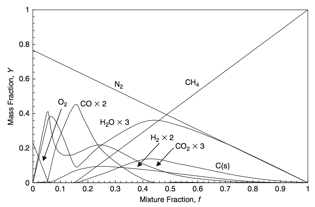
Fig. 5.16 The major species concentrations for a mixture fraction model with 11 species for the methane combustion. Source: [YY09].

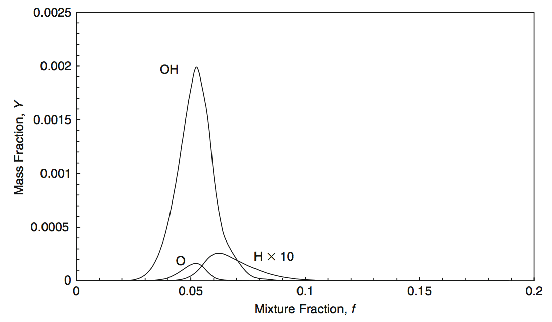
Fig. 5.17 The minor species concentrations for a mixture fraction model with 11 species for the methane combustion. Source: [YY09].

An example for a measurement of the species concentration and temperature as a function of the mixture fraction for a hydrogen-nitrogen mixture fuel is shown in Fig. 5.18.

Fig. 5.18 Measured concentration and temperature values for a laminar (subfigure a and b) and a turbulent flame (subfigures c and d). Source: [YTM20].

The mixture fraction itself is a conserved scalar and is advected by the flow. Thus its transport equation is the following

\[ \mf \partial_t \left(\rho\, f\right) + \nabla\cdot(\rho\vec{v}\,f) = \nabla \cdot \frac{\mu}{Sc} \nabla f \quad . \]

Here the diffusion is approximation is based on the viscosity and the Schmidt number (\(\mf Sc\)). In case of a turbulence modell, the according effective values have to be used.

Finite Rate Formulation

To allow for finite rate reactions, the concentrations of all involved species must be computed.

In a system with \(\mf N\) species, the mass fractions \(\mf Y_i\) are given by

\[ \mf Y_i = \frac{m_i}{M}\quad \mbox{with the total mass} \quad M = \sum_{i=1}^N m_i \quad \mbox{and}\quad \sum_{i=1}^N Y_i = 1 \]

The volume fraction \(\mf X_i\) is defined in an alalogous way.

The conservation equation for the i-th species takes the following form

\[ \mf \partial_t (\rho Y_i) + \nabla\cdot(\rho\vec{v} Y_i) = \nabla\cdot(\rho D_i \nabla Y_i) + R_i \]

with the diffusion coefficient \(\mf D_i\) and the reaction rate \(\mf R_i\).

In general the diffusion coefficient \(\mf D_i\) is different for each species is different. However, a commonly used approximation is to assume that all species have the same diffusion properties

\[ \mf \rho D_i = \frac{\mu}{Sc_i} \approx \frac{\mu}{Sc} \]

Therefore a global \(\mf D\) is found with a usually prescribed Schmidt number of 0.7, which allows to compute the dynamics of multiple species as one. This is the lumped species approach. In the lumped species approach, related primitive species \(\mf Y_\alpha\), e.g. nitrogen, oxygen, and carbon dioxide, are transported together. The classification into three lumped species \(\mf Z_A\) (air), \(\mf Z_F\) (fuel) and \(\mf Z_P\) (products) leads in the case of methane combustion

\[ \mf CH_4 + 2 \left(O_2 + \frac{0.79}{0.21} N_2\right) \rightarrow CO_2 + 2H_2O + 2\frac{0.79}{0.21}N_2 \]

to the following relation

\[\begin{split} \mf \left(\begin{array}{ccc} 0.77 & 0.00 & 0.73 \\ 0.23 & 0.00 & 0.00 \\ 0.00 & 1.00 & 0.00 \\ 0.00 & 0.00 & 0.15 \\ 0.00 & 0.00 & 0.12 \end{array}\right) \cdot \left(\begin{array}{c} Z_A \\ Z_F \\ Z_P\end{array}\right) = \left(\begin{array}{c} Y_{N_2} \\ Y_{O_2} \\ Y_{CH_4} \\ Y_{CO_2} \\ Y_{H_2O}\end{array}\right) \end{split}\]

This approach allows to significantly reduce the cost of the computation of the transport process. The transport of scalars is an advection-diffusion equation including source terms. In the case of the lumped species \(\mf Z_\alpha\) it takes the following form:

\[ \mf \partial_t (\rho Z_\alpha) + \nabla\cdot\left(\rho Z_\alpha \vec{v}\right) = \nabla\cdot\left(\rho D_\alpha \nabla Z_\alpha\right) + \dot{m}_\alpha + \dot{m}_{b, \alpha} \]

with the diffusion coefficient \(\mf D_\alpha\) and the mass sources \(\mf \dot{m}_\alpha\). The solution of this set of equations must satisfy the realizability condition, which is

\[ \mf Y_\alpha \geq 0 \quad \text{and} \quad \sum Y_\alpha = 1 \quad . \]

The zoo of possible reactions may be formalized into a general stoichiometric equation for the j-th reaction (with a total of \(\mf N\) species):

\[ \mf \sum_{i=1}^N \nu_{i,j}' C_{i} \ \ \underset{k_{b,j}}{\stackrel{k_{f,j}}{\rightleftharpoons}} \ \ \sum_{i=1}^N \nu_{i,j}'' C_{i} \]

with \(\mf \nu'\) and \(\mf \nu''\) being the stoichiometric coefficients for the reactants and products.

The reaction rate for the j-th reaction is therefore

\[ \mf R_j \propto k_{f,j} \prod_{i+1}^N C_i^{n_{i,j}'} - k_{b,j} \prod_{i+1}^N C_i^{n_{i,j}''} \]

with the reaction rates in forward direction \(\mf k_{f,j}\) and backward direction \(\mf k_{b,j}\), as well as the rate exponents \(\mf n_{i,j}'\) and \(\mf n_{i,j}''\). This equation misses the third body effects, which set the proportionality constant.

In the case of the reaction

\[ \mf CO + OH \rightleftharpoons CO_2 + H \]

the stoichiometric coefficients are all unity. This is also true for the rate exponents. Therefore

\[ \mf R = k_f C_{CO}C_{OH} - k_b C_{CO_2}C_{H} \]

The forward reaction rate may be computed using Arrhenius expression and the backward rate is given by an equilibrium condition.