fdsreader Module#
In order to analyse simulation data computed by FDS with Python, we have developed the Python module fdsreader. Its aim is to read most data output formats generated by FDS and map them to Python data structures.
It is freely available and open source. The source code is hosted at GitHub: FireDynamics/fdsreader and there is also an API documentation.
import matplotlib
import matplotlib.pyplot as plt
plt.rcParams['figure.figsize'] = (6, 4)

import numpy as np

from IPython.display import display
from PIL import Image
Installation#
The fdsreader module can be installed via pip (see also the GitHub repository):
pip install fdsreader
However, it is already installed on all JupyterLab instances used for this lecture.
Basic Demo Data Set#
To demonstrate the usage of the fdsreader module, a simple FDS scenario (Steckler compartment) is utilized. Here, only a single mesh is used and only the fundamental data types are involved.
Full FDS input file
&HEAD CHID='StecklerExample', TITLE='Example of a Steckler case, with 3/6 door' /

&TIME T_END=1800.0 /
&DUMP NFRAMES=1800 /

&MISC BNDF_DEFAULT=F /

# ---------------------------------------
# Computational domain
# ---------------------------------------

&MESH ID  = 'Domain_Simple',
      IJK = 40,28,22,
      XB  = -1.40,2.60,-1.40,1.40,0.00,2.20 /


# ---------------------------------------
# Open boundary conditions
# ---------------------------------------

&VENT MB='XMAX', SURF_ID='OPEN' /

&VENT ID      = 'OpenCeiling',
      SURF_ID = 'OPEN',
      XB      = 1.51,2.60,-1.40,1.40,2.20,2.20 /
&VENT ID      = 'OpenLeft',
      SURF_ID = 'OPEN',
      XB      = 1.51,2.60,-1.40,-1.40,0.00,2.20 /
&VENT ID      = 'OpenRight',
      SURF_ID = 'OPEN',
      XB      = 1.51,2.60,1.40,1.40,0.00,2.20 /

# ---------------------------------------
# Gas burner: propane
# ---------------------------------------

&SPEC ID = 'PROPANE' /

&REAC FUEL       = 'PROPANE',
      SOOT_YIELD = 0.022 /

# HRR: 62.9 kW
&SURF ID         = 'BURNER',
      HRRPUA     = 393.74999999999994,
      SPEC_ID(1) = 'PROPANE'
      COLOR      = 'RASPBERRY' /

&OBST SURF_ID = 'INERT',
      XB      = -0.2, 0.2, -0.2, 0.2, 0.0, 0.2 /

&VENT SURF_ID = 'BURNER',
      XB      = -0.2, 0.2, -0.2, 0.2, 0.2, 0.2 /


# ---------------------------------------
# Surface definition (boundary conditions)
# ---------------------------------------

&SURF ID                      = 'Wall Lining',
      COLOR                   = 'BEIGE',
      DEFAULT                 = T,
      THICKNESS(1:1)          = 0.0254,
      MATL_ID(1,1:1)          = 'MARINITE',
      MATL_MASS_FRACTION(1,1) = 1.0 /


&MATL ID            = 'MARINITE'
      EMISSIVITY    = 0.9
      DENSITY       = 737.
      SPECIFIC_HEAT = 1.2
      CONDUCTIVITY  = 0.12 /


# ---------------------------------------
# Geometrical Structure
# ---------------------------------------

&OBST ID        = 'Ceiling',
      SURF_ID   = 'Wall Lining',
      BNDF_OBST = T,
      XB        = -1.51,1.51,-1.51,1.51,2.20,2.31 /

&OBST ID      = 'WallFront',
      SURF_ID = 'Wall Lining'
      XB      = 1.40,1.51,-1.51,1.51,0.00,2.20 /

&OBST ID      = 'WallRight',
      SURF_ID = 'Wall Lining',
      BNDF_OBST = T,
      XB      = -1.40,1.40,1.40,1.51,0.00,2.20 /

# Cut out for door
&HOLE ID = 'WallFront.001'
      XB=1.4050,1.5150,-0.2000,0.2000,0.0000,1.8000 /


# ---------------------------------------
# Analytics
# ---------------------------------------

&SLCF PBX      = 0.00
      QUANTITY = 'TEMPERATURE' /
&SLCF PBY      = 0.00
      QUANTITY = 'TEMPERATURE' /

&SLCF PBX           = 0.00
      QUANTITY      = 'W-VELOCITY' /
&SLCF PBY           = 0.00
      QUANTITY      = 'U-VELOCITY' /

&SLCF PBZ           = 1.80
      QUANTITY      = 'W-VELOCITY' /

&BNDF QUANTITY      = 'WALL TEMPERATURE',
      CELL_CENTERED = T /

&DEVC ID       = 'Temp_Door_Low',
      QUANTITY = 'TEMPERATURE',
      XYZ      = 1.45, 0.05, 0.1 /

&DEVC ID       = 'Temp_Door_Mid',
      QUANTITY = 'TEMPERATURE',
      XYZ      = 1.45, 0.05, 1.0 /

&DEVC ID       = 'Temp_Door_High',
      QUANTITY = 'TEMPERATURE',
      XYZ      = 1.45, 0.05, 1.65 /

&TAIL/
Precomputed simulation data
Open the Data Set#
First the fdsreader module needs to be loaded:
import fdsreader
The version of (any) module can be checked with the __version__ variable:
fdsreader.__version__
'1.9.1'
Next, the reader needs to be pointed to the directory, which contains the simulation data, especailly the smokeview file.
# define the path to the data
path_to_data = 'data/fdsreader/example_01/rundir'

sim = fdsreader.Simulation(path_to_data)
The Simulation object sim contains now all the information and data about the simulaiton output:
sim
Simulation(chid=StecklerExample,
           meshes=1,
           obstructions=4,
           slices=5,
           smoke_3d=3,
           devices=4)
The variable sim contains information about the mesh (MESH), four slices (SLCF) and four point measurements (DEVC). The additional device – there were just three defined in the FDS input file – is the time column.
Tip
You can use the autocomplete function in Jupyter. This way you can quickly see available data structures and functions, especially in complex data types as the Simulation object.
Device Data#
The simplest data set is the output of the DEVC directives. The available data and meta information can be directly printed:
# short reference for convinience, i.e. `devc` contains all devices
devc = sim.devices
print(devc)
[Device(id='Time', xyz=(0.0, 0.0, 0.0), quantity=Quantity('TIME')),
Device(id='Temp_Door_Low', xyz=(1.45, 0.05, 0.1), quantity=Quantity('TEMPERATURE')),
Device(id='Temp_Door_Mid', xyz=(1.45, 0.05, 1.0), quantity=Quantity('TEMPERATURE')),
Device(id='Temp_Door_High', xyz=(1.45, 0.05, 1.65), quantity=Quantity('TEMPERATURE'))]
The Device class contains all relevant information, see device documentation.
for i in devc:
    print(f"ID: {i.id},\t quantity: {i.quantity_name}, \t position: {i.position}")
ID: Time,	 quantity: TIME, 	 position: (0.0, 0.0, 0.0)
ID: Temp_Door_Low,	 quantity: TEMPERATURE, 	 position: (1.45, 0.05, 0.1)
ID: Temp_Door_Mid,	 quantity: TEMPERATURE, 	 position: (1.45, 0.05, 1.0)
ID: Temp_Door_High,	 quantity: TEMPERATURE, 	 position: (1.45, 0.05, 1.65)
Tip
Autocomplete works also for the dictionary keys ;-)
Individual devices, including the time column, are accessable as dictironary entries using their ID as key. The data of each individual device (Device.data) is stored as a numpy array:
type(devc['Temp_Door_Mid'].data)
numpy.ndarray
The length matches the expected value, i.e. 1801, as the simulation time was \(\mf 1800\ s\) and the divices were writen out every second, including the initial time step, here at \(\mf t=0\ s\).
len(devc['Time'].data)
1801
A raw look at the data (Device.data):
devc['Temp_Door_Mid'].data
array([ 20.      ,  20.002083,  20.034418, ..., 105.32822 , 114.82179 ,
       115.01705 ], dtype=float32)
The device data can be also visualised with matplotlib:
# create the plot
plt.plot(devc['Time'].data, devc['Temp_Door_High'].data)

# label the axes
plt.xlabel("time / s")
devc_id = devc['Temp_Door_High'].id
devc_q = devc['Temp_Door_High'].quantity_name
devc_u = devc['Temp_Door_High'].unit
plt.ylabel(f"{devc_q} ({devc_id}) / {devc_u}")

# add a grid
plt.grid()

# save output to file
plt.savefig('figs/device_demo_01.svg', bbox_inches='tight')

plt.close()

Fig. 38 Visualization of the data of one of the devices.#
In the same manner a set of devices can be plotted at once. Like all devices with names starting with Temp_:
# loop over all devices
for i in devc:

    # consider only devices with an ID that starts with 'Temp_'
    if not i.id.startswith('Temp_'):
        continue

    plt.plot(devc["Time"].data, i.data, label=i.id)

plt.legend()
plt.xlabel("time / s")
plt.ylabel('temperature / $^\circ$C')
plt.grid()

# save output to file
plt.savefig('figs/device_demo_02.svg', bbox_inches='tight')

plt.close()

Fig. 39 Visualization of the data of a set of devices.#
HRR Data#
In the same fashion as the DEVC data, the data written to the HRR file can be directly accessed. It is not stored in the devices but in the hrr element of the Simulation object.
plt.plot(sim.hrr['Time'], sim.hrr['HRR'], label='heat release from fire')

plt.plot(sim.hrr['Time'], sim.hrr['Q_RADI'], label='radiative')
plt.plot(sim.hrr['Time'], sim.hrr['Q_COND'], label='conductive')
plt.plot(sim.hrr['Time'], sim.hrr['Q_CONV'], label='convective')

plt.plot(sim.hrr['Time'],
         sim.hrr['HRR'] + sim.hrr['Q_RADI'] + sim.hrr['Q_COND'] + sim.hrr['Q_CONV'],
         color='grey', label='sum', zorder=0)

plt.xlabel('time / s')
plt.ylabel('heat flow rate / kW')
plt.legend()

plt.grid()

# save output to file
plt.savefig('figs/hrr_demo_01.svg', bbox_inches='tight')
plt.close()

Fig. 40 Visualization of a set of columns from the HHR file.#
Slice Data#
Data generated by SLCF directives span over two or three spatial dimensions plus the time dimension. Besides that, they can be distributed across multiple meshes.
The data of a slice is stored for each mesh individually. In this simple example, there is only a single mesh, yet for formal consistency it still needs to be referred.
The data sturcutre is as follows
sim.slices[sliceid][meshid].data[timestep, direction1, direction2]
where sliceid is just the index of the slice, meshid is the index of the mesh, here in this example 0, and the reference to the data is given by the time step id and then the two spatial indices (for two dimensional slices).
In general there are multiple slice objects available:
# print available slice data
for slice in sim.slices:
    print(f"Slice Type [2D/3D]: {slice.type}\n  Quantity: {slice.quantity.name}\n",
          f" Physical Extent: {slice.extent}\n  Orientation [1/2/3]: {slice.orientation}\n")
Slice Type [2D/3D]: 2D
  Quantity: TEMPERATURE
  Physical Extent: Extent([0.00, 0.00] x [-1.40, 1.40] x [0.00, 2.20])
  Orientation [1/2/3]: 1

Slice Type [2D/3D]: 2D
  Quantity: TEMPERATURE
  Physical Extent: Extent([-1.40, 2.60] x [0.00, 0.00] x [0.00, 2.20])
  Orientation [1/2/3]: 2

Slice Type [2D/3D]: 2D
  Quantity: W-VELOCITY
  Physical Extent: Extent([0.00, 0.00] x [-1.40, 1.40] x [0.00, 2.20])
  Orientation [1/2/3]: 1

Slice Type [2D/3D]: 2D
  Quantity: U-VELOCITY
  Physical Extent: Extent([-1.40, 2.60] x [0.00, 0.00] x [0.00, 2.20])
  Orientation [1/2/3]: 2

Slice Type [2D/3D]: 2D
  Quantity: W-VELOCITY
  Physical Extent: Extent([-1.40, 2.60] x [-1.40, 1.40] x [1.80, 1.80])
  Orientation [1/2/3]: 3
There are multiple ways to find the right slice in the set of all slices. One way is to filter for a quantity using the filter_by_quantity function or choose a slice by its ID.
# get the W-VELOCITY slice(s)
w_slice = sim.slices.filter_by_quantity("W-VELOCITY")
print(w_slice)
SliceCollection([Slice([2D] quantity=Quantity('W-VELOCITY'), cell_centered=False, extent=Extent([0.00, 0.00] x [-1.40, 1.40] x [0.00, 2.20]), extent_dirs=('y', 'z'), orientation=1),
Slice([2D] quantity=Quantity('W-VELOCITY'), cell_centered=False, extent=Extent([-1.40, 2.60] x [-1.40, 1.40] x [1.80, 1.80]), extent_dirs=('x', 'y'), orientation=3)])
Another way is to select a slice based on its distance to a given point.
# select slice, by its distance to a given point
slc = w_slice.get_nearest(x=1, z=2)
print(slc)
Slice([2D] quantity=Quantity('W-VELOCITY'), cell_centered=False, extent=Extent([-1.40, 2.60] x [-1.40, 1.40] x [1.80, 1.80]), extent_dirs=('x', 'y'), orientation=3)
To access the actual slice data, the actual mesh and a point in time needs to be specified. In this example, there is only one mesh, thus the index is 0. The function get_nearest_timestemp helps to find the right time index.
# choose and output the time step, next to t=75 s
it = slc.get_nearest_timestep(25)
print(f"Time step: {it}")
print(f"Simulation time: {slc.times[it]}")
Time step: 25
Simulation time: 25.02111
The following example illustrates the visualisation of the data and steps needed to adjust the representation. The needed adjustments are due to the data orientation expected by the imshow function.
# choose the temperature slice in y-direction
slc = sim.slices.filter_by_quantity('TEMPERATURE').get_nearest(x=3, y=0)
print(slc)
# only one mesh
slc_data = slc[0].data
print(slc_data)
Slice([2D] quantity=Quantity('TEMPERATURE'), cell_centered=False, extent=Extent([-1.40, 2.60] x [0.00, 0.00] x [0.00, 2.20]), extent_dirs=('x', 'z'), orientation=2)
[[[ 20.        20.        20.       ...  20.        20.        20.      ]
  [ 20.        20.        20.       ...  20.        20.        20.      ]
  [ 20.        20.        20.       ...  20.        20.        20.      ]
  ...
  [ 20.        20.        20.       ...  20.        20.        20.      ]
  [ 20.        20.        20.       ...  20.        20.        20.      ]
  [ 20.        20.        20.       ...  20.        20.        20.      ]]

 [[ 20.030926  20.031328  20.032204 ...  20.001385  20.001268  20.00117 ]
  [ 20.030703  20.031597  20.033634 ...  20.001493  20.001345  20.001238]
  [ 20.031723  20.033785  20.038801 ...  20.001757  20.001535  20.001389]
  ...
  [ 20.006077  20.004908  20.002953 ...  20.001383  20.001154  20.00104 ]
  [ 20.005085  20.004053  20.00236  ...  20.00129   20.001116  20.001026]
  [ 20.004608  20.003656  20.0021   ...  20.00125   20.001104  20.001026]]

 [[ 20.12404   20.126698  20.133305 ...  20.026028  20.02525   20.025595]
  [ 20.116137  20.11882   20.12633  ...  20.02626   20.025606  20.02608 ]
  [ 20.114033  20.117645  20.128752 ...  20.02802   20.027351  20.027908]
  ...
  [ 20.018784  20.016739  20.013128 ...  20.00563   20.004776  20.004353]
  [ 20.015898  20.014067  20.010876 ...  20.005054  20.004427  20.004118]
  [ 20.01441   20.012737  20.00983  ...  20.004791  20.004278  20.00403 ]]

 ...

 [[ 44.00391   43.917053  43.920734 ... 143.89009  142.69537  142.16621 ]
  [ 44.004223  43.863914  43.708996 ... 143.29715  142.09953  141.6622  ]
  [ 43.81018   43.64982   43.4085   ... 142.64955  141.90448  141.75969 ]
  ...
  [ 20.284891  20.19156   20.076902 ...  90.631195  78.81051   72.00585 ]
  [ 20.218634  20.140545  20.047134 ...  56.04536   43.176456  39.645744]
  [ 20.151264  20.09307   20.028439 ...  34.67456   27.534237  27.970665]]

 [[ 45.228874  45.115242  44.938766 ... 150.18481  150.12732  149.83371 ]
  [ 44.492287  44.350613  44.180614 ... 149.79759  150.0778   149.77635 ]
  [ 43.646873  43.590538  43.562504 ... 147.7298   148.82109  149.29768 ]
  ...
  [ 20.281096  20.186028  20.071451 ... 106.69953   93.09295   83.79199 ]
  [ 20.205025  20.13359   20.046276 ...  80.62758   71.11945   62.30358 ]
  [ 20.16152   20.102564  20.033293 ...  65.56552   56.724525  46.839134]]

 [[ 42.762764  42.892406  42.67096  ... 146.0912   145.20709  144.58104 ]
  [ 43.14627   43.263447  43.141045 ... 145.02187  144.6713   143.69063 ]
  [ 43.753468  43.769325  43.798447 ... 141.0417   142.32797  141.77148 ]
  ...
  [ 20.268656  20.194078  20.08938  ...  72.89162   70.64532   65.348694]
  [ 20.206676  20.136755  20.052374 ...  59.554634  49.809177  42.573883]
  [ 20.180956  20.111738  20.035168 ...  48.16472   36.145966  31.134487]]]
# Initial visualasation of the data at time t=50 s
it = slc.get_nearest_timestep(50)
plt.imshow(slc_data[it]);

# save output to file
plt.savefig('figs/slice_imshow_01.svg', bbox_inches='tight')
plt.close()

Fig. 41 Visualization of a slice.#
# Access the transpose data using ndarray.T and set the origin of the output
plt.imshow(slc_data[it].T, origin='lower');

# save output to file
plt.savefig('figs/slice_imshow_02.svg', bbox_inches='tight')
plt.close()

Fig. 42 Visualization of a slice.#
# Finally, also the extend is specified to move from index to physical space
# Additionally, the maximal value is set using the vmax argument
plt.imshow(slc_data[it].T,
           origin='lower',
           vmax=200,
           extent=slc.extent.as_list())
plt.colorbar(label='temperature / C', orientation='horizontal');
plt.xlabel('x coordinate / m')
plt.ylabel('z coordinate / m')

# save output to file
plt.savefig('figs/slice_imshow_03.svg', bbox_inches='tight')
plt.close()

Fig. 43 Visualization of a slice.#
Obstructions can be visualised using masks, i.e. the data points which lie inside an obstacle will be marked non-valid as an not-a-number (nan) value.
# Example for a multi plot
list_t = [0, 50, 100, 200, 300, 400]
fig, axs = plt.subplots(2,3, sharex=True, sharey=True)
for i in range(len(list_t)):
    it = slc.get_nearest_timestep(list_t[i])
    axs.flat[i].imshow(slc_data[it].T,
                       vmin=20,
                       vmax=400,
                       origin='lower',
                       extent=slc.extent.as_list())
    axs.flat[i].set_title(f"t={slc.times[it]:.1f}")

# save output to file
plt.savefig('figs/slice_imshow_04.svg', bbox_inches='tight')
plt.close()

Fig. 44 Visualization of a slice.#
# Example for a plot of all slice quantities at a given point in time
it = sim.slices[0].get_nearest_timestep(100)
fig_count=0
for slc in sim.slices:
    plt.imshow(slc[0].data[it].T,
               origin='lower',
               extent=slc.extent.as_list())
    q = slc.quantity.quantity
    u = slc.quantity.unit
    plt.xlabel(f'{slc.extent_dirs[0]} / m')
    plt.ylabel(f'{slc.extent_dirs[1]} / m')
    plt.colorbar(label=f"{q} / {u}")
    # save output to file
    plt.savefig(f'figs/slice_multi_{fig_count:02d}.svg', bbox_inches='tight')
    fig_count += 1
    plt.close()

Fig. 45 Visualization of a slice.#

Fig. 46 Visualization of a slice.#

Fig. 47 Visualization of a slice.#

Fig. 48 Visualization of a slice.#

Fig. 49 Visualization of a slice.#
Advanced Demo#
In contrast to the above example, the computational domain is split into two meshes.
Full FDS input file
&HEAD CHID='StecklerExample', TITLE='Example of a Steckler case, with 3/6 door' /

&TIME T_END=1800.0 /
&DUMP NFRAMES=1800 /

&MISC BNDF_DEFAULT=F /

# ---------------------------------------
# Computational domain
# ---------------------------------------

&MESH ID  = 'Domain_A',
      IJK = 20,28,22,
      XB  = -1.40,0.60,-1.40,1.40,0.00,2.20 /

&MESH ID  = 'Domain_B',
      IJK = 20,28,22,
      XB  = 0.60,2.60,-1.40,1.40,0.00,2.20 /


# ---------------------------------------
# Open boundary conditions
# ---------------------------------------

&VENT MB='XMAX', SURF_ID='OPEN' /

&VENT ID      = 'OpenCeiling',
      SURF_ID = 'OPEN',
      XB      = 1.51,2.60,-1.40,1.40,2.20,2.20 /
&VENT ID      = 'OpenLeft',
      SURF_ID = 'OPEN',
      XB      = 1.51,2.60,-1.40,-1.40,0.00,2.20 /
&VENT ID      = 'OpenRight',
      SURF_ID = 'OPEN',
      XB      = 1.51,2.60,1.40,1.40,0.00,2.20 /


# ---------------------------------------
# Gas burner: propane
# ---------------------------------------

&SPEC ID = 'PROPANE' /

&REAC FUEL       = 'PROPANE',
      SOOT_YIELD = 0.022 /

# HRR: 62.9 kW
&SURF ID         = 'BURNER',
      HRRPUA     = 393.74999999999994,
      SPEC_ID(1) = 'PROPANE'
      COLOR      = 'RASPBERRY' /

&OBST SURF_ID = 'INERT',
      XB      = -0.2, 0.2, -0.2, 0.2, 0.0, 0.2 /

&VENT SURF_ID = 'BURNER',
      XB      = -0.2, 0.2, -0.2, 0.2, 0.2, 0.2 /


# ---------------------------------------
# Surface definition (boundary conditions)
# ---------------------------------------

&SURF ID                      = 'Wall Lining',
      COLOR                   = 'BEIGE',
      DEFAULT                 = T,
      THICKNESS(1:1)          = 0.0254,
      MATL_ID(1,1:1)          = 'MARINITE',
      MATL_MASS_FRACTION(1,1) = 1.0 /


&MATL ID            = 'MARINITE'
      EMISSIVITY    = 0.9
      DENSITY       = 737.
      SPECIFIC_HEAT = 1.2
      CONDUCTIVITY  = 0.12 /


# ---------------------------------------
# Geometrical Structure
# ---------------------------------------

&OBST ID        = 'Ceiling',
      SURF_ID   = 'Wall Lining',
      BNDF_OBST = T,
      XB        = -1.51,1.51,-1.51,1.51,2.20,2.31 /

&OBST ID      = 'WallFront',
      SURF_ID = 'Wall Lining'
      XB      = 1.40,1.51,-1.51,1.51,0.00,2.20 /

&OBST ID      = 'WallRight',
      SURF_ID = 'Wall Lining',
      BNDF_OBST = T,
      XB      = -1.40,1.40,1.40,1.51,0.00,2.20 /

# Cut out for door
&HOLE ID = 'WallFront.001'
      XB=1.4050,1.5150,-0.2000,0.2000,0.0000,1.8000 /


# ---------------------------------------
# Analytics
# ---------------------------------------

&SLCF PBX      = 0.00
      QUANTITY = 'TEMPERATURE' /
&SLCF PBY      = 0.00
      QUANTITY = 'TEMPERATURE' /

&SLCF PBX           = 0.00
      QUANTITY      = 'W-VELOCITY' /
&SLCF PBY           = 0.00
      QUANTITY      = 'U-VELOCITY' /

&SLCF PBZ           = 1.80
      QUANTITY      = 'W-VELOCITY' /

&BNDF QUANTITY      = 'WALL TEMPERATURE',
      CELL_CENTERED = T /

&DEVC ID       = 'Temp_Door_Low',
      QUANTITY = 'TEMPERATURE',
      XYZ      = 1.45, 0.05, 0.1 /

&DEVC ID       = 'Temp_Door_Mid',
      QUANTITY = 'TEMPERATURE',
      XYZ      = 1.45, 0.05, 1.0 /

&DEVC ID       = 'Temp_Door_High',
      QUANTITY = 'TEMPERATURE',
      XYZ      = 1.45, 0.05, 1.65 /

&TAIL/
Precomputed simulation data
# define the path to the data
path_to_data = 'data/fdsreader/example_02/rundir'

sim = fdsreader.Simulation(path_to_data)
print(sim)
Simulation(chid=StecklerExample,
           meshes=2,
           obstructions=4,
           slices=5,
           smoke_3d=3,
           devices=4)
Multi Mesh Slices#
First, one of the slices is selected, e.g. the temperature slice normal to y
slc = sim.slices.filter_by_quantity('TEMPERATURE').get_nearest(x=2, y=0)
print(slc)
Slice([2D] quantity=Quantity('TEMPERATURE'), cell_centered=False, extent=Extent([-1.40, 2.60] x [0.00, 0.00] x [0.00, 2.20]), extent_dirs=('x', 'z'), orientation=2)
Each slice records in which meshes it is present. In this case, these are just two.
slc.meshes
[Mesh(id="Domain_A", extent=Extent([-1.40, 0.60] x [-1.40, 1.40] x [0.00, 2.20]), dimension=Dimension(21, 29, 23)),
 Mesh(id="Domain_B", extent=Extent([0.60, 2.60] x [-1.40, 1.40] x [0.00, 2.20]), dimension=Dimension(21, 29, 23))]
The data strucutre of a slice is, that it consists of a set of sub-slices, one for each mesh. These are of variable size, depending on the mesh structure. The sub-slices can be individually accessed.
for m in slc.meshes:
    print(slc.get_subslice(m))
SubSlice(shape=(21, 23), mesh=Domain_A, extent=Extent([-1.40, 0.60] x [0.00, 0.00] x [0.00, 2.20]))
SubSlice(shape=(21, 23), mesh=Domain_B, extent=Extent([0.60, 2.60] x [0.00, 0.00] x [0.00, 2.20]))
it = slc.get_nearest_timestep(100)
fig, axs = plt.subplots(1,2)
ax_count=0
for m in slc.meshes:
    s = slc.get_subslice(m)
    axs.flat[ax_count].imshow(s.data[it].T,
                              origin='lower',
                              extent=s.extent.as_list(),
                              vmax=200)
    axs.flat[ax_count].set_xlabel(f'{slc.extent_dirs[0]} / m')
    axs.flat[ax_count].set_ylabel(f'{slc.extent_dirs[1]} / m')
    ax_count += 1

plt.tight_layout()
# save output to file
plt.savefig('figs/multi_slice_separate.svg', bbox_inches='tight')
plt.close()

Fig. 50 Individual visualization of slices on two meshes.#
In order to merge the subslices, the to_global function can be used.
gslice, gcoord = slc.to_global(return_coordinates=True)
print(type(gslice))
print(gslice.shape)
<class 'numpy.ndarray'>
(1801, 41, 23)
The resulting data structure can now be used the same way as the one mesh slices. Yet, the meta data needs to be drawn from the original slice object, as the result of to_global is a plain numpy array.
plt.imshow(gslice[it].T,
           origin='lower',
           extent=slc.extent.as_list(),
           vmax=200)
plt.xlabel(f'{slc.extent_dirs[0]} / m')
plt.ylabel(f'{slc.extent_dirs[1]} / m')
plt.colorbar(orientation='horizontal', label=f'{slc.quantity.name} / {slc.quantity.unit}')

# save output to file
plt.savefig('figs/multi_slice_global.svg', bbox_inches='tight')
plt.close()

Fig. 51 Visualization of a global, i.e. merged, slice.#
Accessing Slice Data#
The data of a slice can be accessed to extract various subsets of data. For example, to create a temperature and x-velocity profile at a given time across the door (in z-direction) can be achieved with the following code.
# get the slice data as global objects
u_slice = sim.slices.filter_by_quantity('U-VELOCITY').get_nearest(x=2, y=0).to_global()
t_slice = sim.slices.filter_by_quantity('TEMPERATURE').get_nearest(x=2, y=0).to_global()
# define the time index
it = sim.slices[0].get_nearest_timestep(100)
fig, ax1 = plt.subplots()
ax2 = ax1.twiny()

# select spatial index (ix) based on physical position (x0)
x0 = 1.25
ix = np.where(gcoord['x'] >= x0)[0][0]

ax1.plot(u_slice[it][ix,:], gcoord['z'], label='x-velocity', color='C0')
ax2.plot(t_slice[it][ix,:], gcoord['z'], label='temperature', color='C1')
ax1.set_xlabel('velocity / m/s', color='C0')
ax2.set_xlabel('temperature / C', color='C1')
ax1.set_ylabel('height / m')
plt.grid()
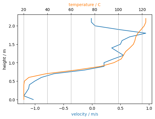
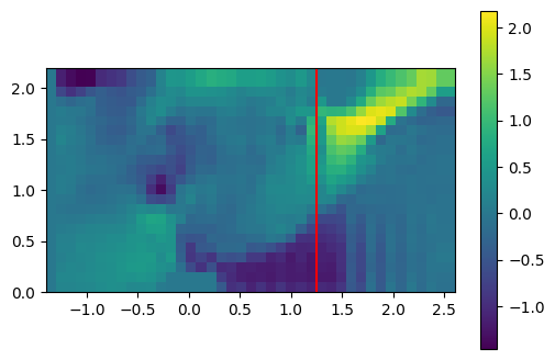
# illustrate the location of the extracted data
plt.imshow(u_slice[it].T,
           origin='lower',
           extent=slc.extent.as_list())
plt.axvline(x=x0, color='red')
plt.colorbar();
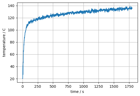
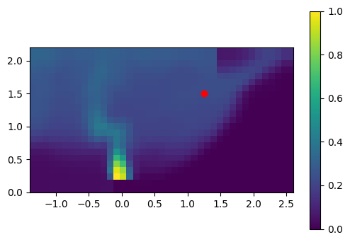
The time evolution of a quantity at a given location is accessed in a similar way.
# select spatial index
x0 = 1.25
z0 = 1.50
ix = np.where(gcoord['x'] >= x0)[0][0]
iy = np.where(gcoord['z'] >= z0)[0][0]

plt.plot(slc.times, t_slice[:, ix, iy])
plt.xlabel('time / s')
plt.ylabel('temperature / C')
plt.grid()
# illustrate the location of the extracted data
plt.imshow(t_slice[it].T,
           origin='lower',
           extent=slc.extent.as_list())
plt.scatter(x0, z0, color='red')
plt.colorbar();
Boundary Data#
In a similar manner as the slice data, the boudary data of obstructions can be accessed. As this data is bound to an obstruction in FDS, it is part of each individual obstruction object.
sim.obstructions
ObstructionCollection([Obstruction(id=1, Bounding-Box=Extent([-0.20, 0.20] x [-0.20, 0.20] x [0.00, 0.20]), SubObstructions=1),
Obstruction(id=2, Bounding-Box=Extent([-1.40, 1.51] x [-1.40, 1.40] x [2.20, 2.20]), SubObstructions=2, Quantities=['temp']),
Obstruction(id=4, Bounding-Box=Extent([-1.40, 1.40] x [1.40, 1.40] x [0.00, 2.20]), SubObstructions=2, Quantities=['temp']),
Obstruction(id=3, Bounding-Box=Extent([1.41, 1.51] x [-0.20, 0.20] x [0.00, 0.00]), SubObstructions=1)])
for o in sim.obstructions:
    print(f'ID: {o.id}; has data: {o.has_boundary_data}')
    if o.has_boundary_data:
        print(f'  orientations: {o.orientations}')
        print(f'  quantities: {o.quantities}')
        print(f'  number of involved meshes: {len(o.meshes)}')
ID: 1; has data: False
ID: 2; has data: True
  orientations: [-3]
  quantities: [Quantity('WALL TEMPERATURE')]
  number of involved meshes: 2
ID: 4; has data: True
  orientations: [-2]
  quantities: [Quantity('WALL TEMPERATURE')]
  number of involved meshes: 2
ID: 3; has data: False
Let’s select the boundary at the ceiling, i.e. the one with orientation -3.
obst = sim.obstructions.get_by_id(2)
print(obst)
Obstruction(id=2, Bounding-Box=Extent([-1.40, 1.51] x [-1.40, 1.40] x [2.20, 2.20]), SubObstructions=2, Quantities=['temp'])
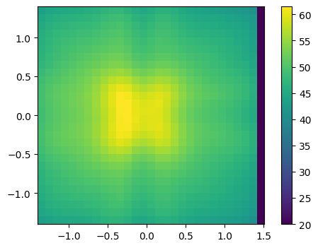
The time step index and the global, due to multiple meshes involved, data structure. The function get_global_boundary_data_arrays needs the quantity and the orientation to create a numpy data object.
obst = sim.obstructions[1]
it = obst.get_nearest_timestep(100)
data = obst.get_global_boundary_data_arrays('WALL TEMPERATURE')[-3]
print(f'shape of the data object: {data.shape}')
shape of the data object: (1801, 29, 28)
plt.imshow(data[it].T,
           origin='lower', extent=obst.bounding_box.as_list())
plt.colorbar()
<matplotlib.colorbar.Colorbar at 0x10ff42da0>
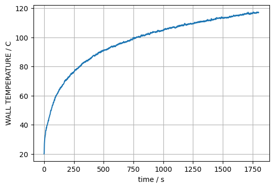
In the same mannor as above, e.g. time series at a given point on the boundary can be created. For a point at the center of the boundary, this could be something like this:
ix = data.shape[1] // 2
iy = data.shape[2] // 2

plt.plot(obst.times, data[:, ix, iy])
plt.xlabel('time / s')
plt.ylabel(f'{obst.quantities[0].name} / {obst.quantities[0].unit}')
plt.grid()