5.4. Wolfhard-Parker Burner#
The Experiments#
In the article A New Technique for the Spectroscopic Examination of Flames at Normal Pressures, published in 1949, H. G. Wolfhard and W. G. Parker presented a gas burner to study laminar diffusion flames. Up to this point, diffusion flames were studied on circular tubes, which makes it difficult to pin-point locations of specific reactions within the flame. For one, because of the circular geometry optical measurement methods collect data from multiple reaction zones. Furthermore, the optical thickness of the individual zones, specifically on the inside of the circle, is very thin.
The Wolfhard-Parker burner produces flat laminar diffusion flames. Thus, facilitates the accurate localisation of the different processes. The burner consists of two rectangular ducts with a cross section of 50 mm by 7 mm, that touch each other at a long edge. One of the ducts provides a fuel gas, while the other provides the oxydiser, here oxygen. Both ducts are located within a third duct, which is used to produce a stream of nitrogen completely surrounding the other two streams. These ducts are located at the bottom of the burner and the combustion products are extracted at the top. The flow velocity of the nitrogen is carefully calibrated, such that the puffing can be prevented and a stable flat flame forms. The flow velocities for the fuel and the oxygen are set to about 20 cm/s. Combustion takes place along the interface between the two main gas streams.
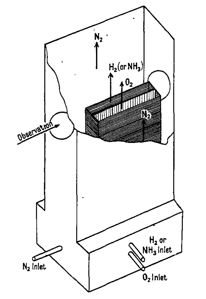
Fig. 5.26 Schematic overview over the Wolfhard-Parker burner.#
Three different fuels have been used: hydrogen (H2), ammonia (NH3) and methane (CH4). It is shown in the article that the flame leans more towards one side of the burner. The reason is described to be the different diffusion rates between the fuels and the oxygen. Thus, it is pointed out that no relationship is made between the dimensions of the burner and the locations in the flame interface.
Measurements have been performed at a height of 12 mm above the burner surface. Primarily, they are spectroscopic measurements of certain reactants of the combustion reaction that can be detected with this technique. For instance, hydrogen cannot be detected with this method, but intermediate products like OH can. Gas temperatures are measured, by inserting a wire, coated with sodium chloride (NaCL) into the gas stream and using the Na-line reversal method. It is found, that for hydrogen the maximum temperature is at about 2800 °C, which is close to the value calculated for the stoichiometric mixture.

Fig. 5.27 Temperature and species distribution in the flat methane-oxygen flame.#
It is described that the fuels form different flames. Hydrogen forms a blue continuum across the reaction zone. Ammonia forms two distinct zones. The zone on the fuel side is a thin yellow layer, while on the oxygen side a blue continuum exists. Both zones are clearly divided by “a dark space”, which is similar to the zone of the methane flame. For the ammonia flame it is reported that, based on the measured spectra, oxygen and NH3 never come into direct contact. The reaction appears to take place only due to intermediate products.
The Simulations#
The Wolfhard-Parker burner is implemented in FDS in a simplified way. No effort is made to implement chemical reactions with the different sub reactions, but it is assumed that the fuel and oxygen react directly. Two vents, for oxidiser and fuel, are positioned in the simulation according to the setup in the experiment. They have both are 50 mm long and 7 mm wide. They are surrounded by a nitrogen flow. It was manually calibrated, such that its flow velocity matches the velocity of the flame. Above the vents a series of devices is located, at a height of 12 mm, to mimic the measurement location described in the article.

Fig. 5.28 Schematic overview over the simulation setup of the Wolfhard-Parker burner.#
Tasks#
Using the DEVC data, create a plot that allows you to determine the quasi-steady state.
Reproduce figure 2 with the DEVC data, including the reaction zone.
Create a contour plot for the gas temperatures over the measurement plane.